RoboCupRescue 2011 - Robot League Team resko@UniKoblenz (Germany)
Dagmar Lang, Marcel Häselich, Martin Prinzen, Simone Bauschke, Alexander Gemmel, Julian Giesen, Ruwen Hahn, Laura Haraké, Paul Reimche, Guido Sonnen, Matthias von Steimker, Susanne Thierfelder, Dietrich Paulus
Active Vision Group; University of Koblenz-Landau
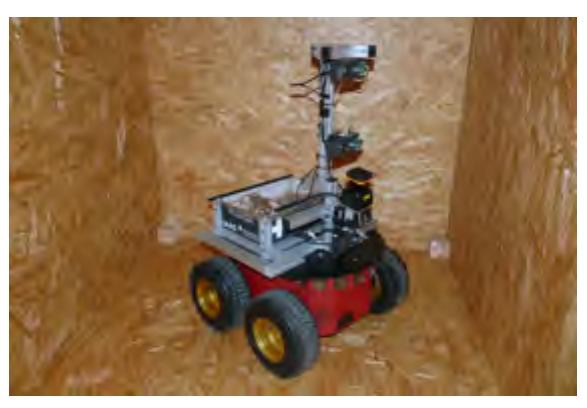
Abstract This describes approach paper the resko@UniKoblenz for the RoboCup Rescue competition Our mobile system Robbie is based on a MobileRobots Pioneer 3 AT. On this platform, an aluminum rack is installed where additional sensors are attached: three color cameras (Philips SPC1330NC), two actively controlled Hokuyo UTM-30LX laser range finders (LRFs), three low-resolution thermal sensors and an inertial measurement unit. The robot can be operated in an autonomous and in a teleoperated mode. The map building is done by the computer automatically by merging the collected LRF data with the odometry information using a Hyper Particle Filter in 2D and in 3D an ICP based approach. The automatic victim detection is based on the thermal sensors and color cameras. Robbie was developed and improved at the University of Koblenz-Landau (Germany) in several practical courses during the last couple of years. The robot was used by the team resko@UniKoblenz at the RoboCup German Open 2007, 2008, 2009 and 2010 and at the RoboCup World Championship 2007 in Atlanta (GA, USA), 2008 in Suzhou (China) and 2009 in Graz (Austria). The team achieved the "Best in Class Autonomy Award" in six of these competitions.
Introduction
The team resko@UniKoblenz is a group of researchers and students from the University of Koblenz-Landau, Germany. In 2011, we are going to compete in the RoboCup Rescue League with our robot Robbie.
1 Team Members and their Contributions
The team resko@UniKoblenz with focus on the RoboCup Rescue league consists of the following members:
- Dagmar Lang: team leader resko, scientific supervisor, SLAM
- Marcel Häselich: project leader, scientific supervisor, senor data fusion
- Martin Prinzen: technical design, programming
- Simone Bauschke: public relations, programming
- Alexander Gemmel: quality assurance, programming
- Julian Giesen: software assistant, programming
- Ruwen Hahn: network administrator, programming
- Laura Haraké: hardware assistant, programming
- Paul Reimche: media, programming
- Guido Sonnen: infrastructure, programming
- Matthias von Steimker: 3D mapping, programming
2 Control method and Human-Robot Interface (HRI)
Our robot navigates through the yellow part of the RoboCup Rescue Arena autonomously. The robot is started by the operator via operator station; afterwards the operator can monitor the robot and the sensor data, which are sent to the operator station via WLAN. In case of emergency, the operator can stop the autonomous mode and teleoperate the robot. If the connection to the operator station gets lost, the robot continues its mission and the victim search. As soon as the connection is re-established, the victim verification on the operator station is triggered.
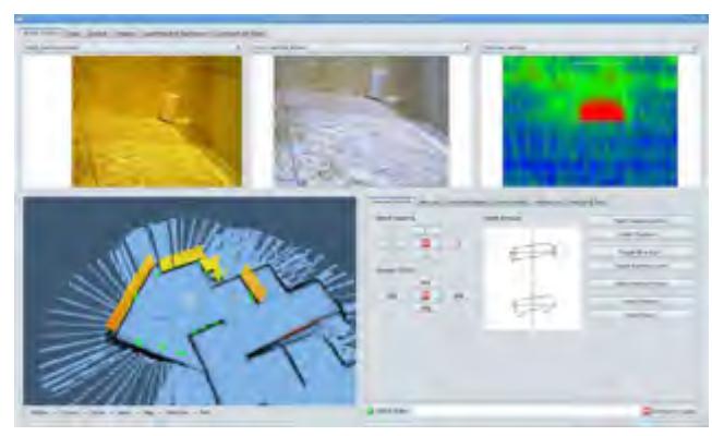
The graphical user interface (GUI) of the operator laptop is shown in Fig. 1b. The human-robot interface is implemented in Qt4, with OpenGL widgets for visualizing easy-to-understand 3D views of the sensor data. The operator surveys all sensor measurements, the color images and the last thermal image on a single screen. The current laser and sonar range readings are merged into the already learned map in the lower left part of the window. In the upper part of the window, the images of the color cameras and the thermal image are shown. The operator can mark the position of victims in the map manually. In the autonomous mode, a dialog pops up when the robot has found a victim. This (potential) victim can then be verified or declined; the position is automatically marked in the map. Additionally, the robot has a blue flashing light that indicates the detection of a victim. This shows the audience that the victim detection was successful.
3 Map generation/printing
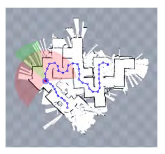
While exploring the environment, the robot automatically generates a map of the building. The map is based on the laser scans and the odometry information. Fig. 2 shows the result of the mapping process.
The data structure to store the map is a single occupancy map. In the context of RoboCup Rescue, the grid usually has a size of $800 \times 800$ cells, which represents a map of an area of $40 \times 40$ meters with a grid cell size of $50 \times 50$ mm. The grid is stored in two planes: one plane counts how often a cell was "seen" by a laser beam. This value is increased either if the laser beam measured the cell as free or as occupied. A second plane stores the information how often a cell was seen as occupied. By dividing these two planes, the occupancy probability for a cell $c^i$ is calculated as the following ratio:
$$p_{\rm occ}(c_i) = \frac{\rm count_{\rm occ}(c_i)}{\rm count_{\rm seen}(c_i)}$$ (1)
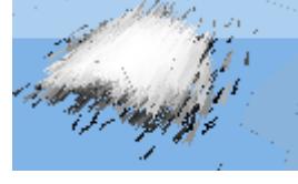
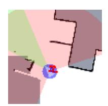
To solve the SLAM problem, we use a particle filter [IB98] with about 1,000 particles [Pel08]. Each particle represents a hypothesis for the pose of the robot in 2D-space: $(x, y, \Theta)^T$. Fig. 3 illustrates the robot pose hypotheses, represented by particles.
The algorithm of the particle filter includes the following steps: resample, drift, measure, and normalize. The result is the most likely pose of the robot when the laser scan was taken. This pose is then used for the map update. An ICP (Iterative Closest Point) scan matcher with different metrics improves the pose estimation (which is the input for the particle filter) that is based on the odometry of the robot.
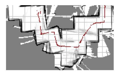
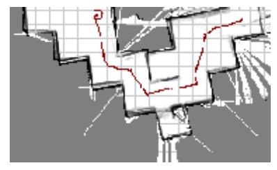
We use a Hyper Particle Filter (HPF) [PP09] – a Particle Filter of Particle Filters – for solving the SLAM problem. Each particle of the HPF contains a standard localization Particle Filter (with a map and a set of particles, that model the belief of the robot pose in this particular map). Using this technique, broken maps are very unlikely. Also, the problem of loop closing is solved (see Fig. 4). The resulting map is displayed in realtime on the operator station. After the mission we can export our map as a GeoTIFF file and hand it to the responders.
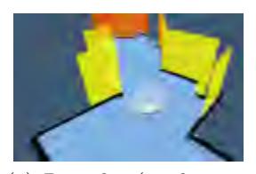
NEW in 2011: In addition to the 2D mapping with the HPF we generate 3D maps. The approach is based on an ICP with 6 DoF to generate the 3D maps as presented on an 3D Logfile of DisasterCity in [PLNP10]. The 3D map provides a much better impression of the terrain, especially for victim localization and detection of step fields, slopes and stairs.
4 Sensors for Navigation and Localization
placeholder
4.1 Odometry data
NEW in 2011: To determine the pose $(x, y, z, \Psi, \Theta, \Phi)^T$ and the acceleration we use an inertial measurement unit (xSens MT-i). The Pioneer 3-AT platform delivers the robot pose $(x, y, \Theta)^T$ based on the readings from the wheel encoders. However, our experiments have shown that the data is quite unreliable, and the errors sum up over time. Therefore this data can only be used to make a rough guess about the robot location and orientation.
4.2 Laser scanner
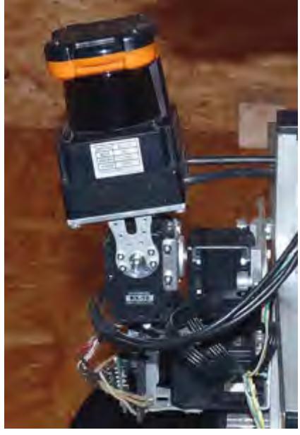
The Hokuyo URG-30LX laser scanner generates 240° scans that measure the distance (up to 5.60 meters) to the closest objects. The resolution of the laser scanner is 0.36°. The operator interface shows these scans with respect to the robot's position. With this information the operator is able to estimate distances to obstacles better than with video images only. The scanner is attached to the front of the robot as shown in Fig. 7a. Detected obstacles (such as walls) are continuously integrated into the map.
3D scans are acquired by tilting the laser scanner forwards, since the laser scanner used is only capable of 2D scans. While the tilt is in progress scans are recorded continuously, as are the reported tilt angles. As soon as the tilt is finished the recorded data is interpolated to extract a 3D point cloud. The attainable vertical resolution of 3D scans depends on the speed and accuracy of the tilt unit and the scanning frequency of the laser scanner.
5 Sensors for Victim Identification
placeholder
5.1 Vision System
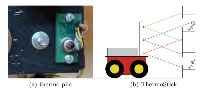
NEW in 2011: Robbie has a vision system with 3 webcams (Philips SPC1330NC) mounted at the front. The webcams are mounted on three different heights shown in Fig. 5b. The different heights enable the robot to detect victims at different heights. Each webcam is mounted next to a thermal sensor as shown in Fig. 5a. Initial victim detection is performed by analyzing the images of the thermal sensors. The camera images are used to verify the victims by the operator.
5.2 Thermal Sensors
NEW in 2011: Heat detection is used to identify victims. Therefore three TPA 81 (see Fig. 5a) infrared piles with a resolution of 8 pixels per pile are used. Each TPA 81 is mounted on a separate rotation unit (Dynamixel RX-10), which are mounted on three different height levels (see Fig. 5b). By rotating all three rotation units simultaneously, a panoramic heat image is created. The resulting heat image is used by the robot to detect victims autonomously based on the heat signatures.
6 Robot Locomotion
The Pioneer 3 AT is a robot equipped with four air-filled tires. They are driven by 4 DC motors (12 volts). We control them by using the programming library (called ARIA) provided by the manufacturer. Apart from the autonomous operation, we implemented a gamepad and a keyboard control.
7 Other Mechanisms
placeholder
7.1 Active Adjustment of the Laser Range Finder
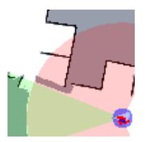
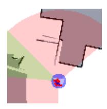
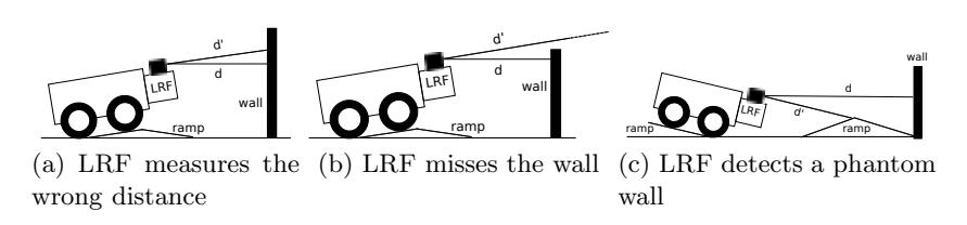
Rescue robots are usually used in unstructured environments with uneven floors and piles of debris. Therefore the sensor readings might be spurious if the sensors are rigidly coupled with the robot. The influence of uneven floor is simulated at the RoboCup using 15° pitch/roll ramps. These ramps influence the LRF data in three different ways:
- The measured distance to an obstacle slightly changes by the factor of $\frac{1}{\cos \alpha}$ compared to the real distance, where $\alpha$ is the pitch angle of the robot relative to the ground.
- The obstacle is not detected at all, since the sensor points above the object.
- "Phantom walls" are detected, since the sensor detects the next pitch ramp as an obstacle.
These problems are illustrated in Fig. 6: While 6a usually adds only a small error (about 1.5% at 10°), 6b and 6c result in inaccurate occupancy maps. Case 6c can cause the robot to avoid a free path, because the map blocks its way with an phantom obstacle. Therefore, we adjust the orientation of the LRF based on the readings from a gravity sensor [Pel07].
7.2 Terrain classification
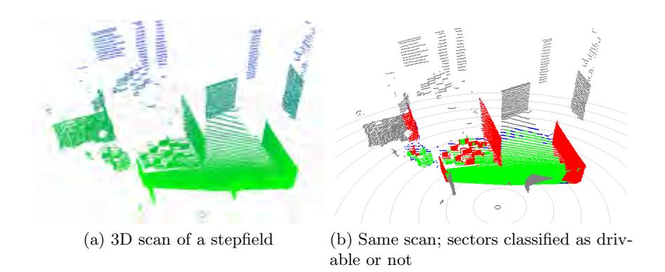
Due to its limited mobility the robot has to avoid rough terrain as simulated with the stepfields in the Orange Arena. Therefore, the robot performs 3D scanning every 2 meters, to locate boundaries to impassable areas. The 3D scans are acquired with same (adjusted) LRF that is used for 2D localization and mapping. The scan is analyzed as follows:
- Each point of the local scan is assigned to a grid cell (of size $100 \times 100$ mm) on the x/y-plane (the x/y-plane is parallel to the ground).
- For each grid cell $c_i$, the variance in z (the height), as well as the the lowest and the highest z value are computed $(\sigma_{z,i}^2, \min_{z,i} \text{ and } \max_{z,i})$. Also, the number of points in each cell is counted $(#_i)$.
- A cell is assigned one of three classes, depending on the precalculated parameters:
$$\operatorname{class}(c_i) = \begin{cases} \operatorname{unknown}, & \text{if } #i < \operatorname{minCnt}, \ \operatorname{occupied}, & \text{if } (\sigma_i^2 > \operatorname{maxVar}) \land ((\operatorname{max}{z,i} - \operatorname{min}_{z,i}) > \operatorname{maxStep}), \ \operatorname{free}, & \text{else.} \end{cases}$$ (2)
- Finally, using the current pose of the robot, the world coordinates of all cells of class occupied are calculated and stored in a 2D grid, the "inaccessible grid": inaccessible(localToWorld(ci)) = true
An example of classified terrain is given in Fig. 8. The values for the thresholds were determined experimentally and are set to: minCnt = 10, maxVar = 18² and maxStep = 80 (all distances in mm).
7.3 Path planning: The Exploration Transform
By combining Yamauchi's frontier based exploration [Yam97] with Zelinsky's path transform (see [Zel88,Zel91]) an elegant solution for the exploration problem can be achieved: the path transform is extended in a way that not the cost of a path to a certain target cell is calculated, but the cost of a path that goes to a close frontier (the boundary between known and unknown areas). The path is not necessarily the shortest and the frontier not necessarily the closest, since the cost is determined by the travel distance and the safety of the path. The overall formula of the Exploration Transform [WP07] is given in (3); it yields for a given cell c the frontier cell that is close and save to reach:
$$\Psi(c) = \min_{c_g \in F} \left( \min_{C \in \chi_c^{c_g}} \left( l(C) + \alpha \sum_{c_i \in C} c_{\text{danger}}(c_i) \right) \right)$$ (3)
with F the set of all frontier cells, $\chi_c^{c_g}$ the set of all paths from c to $c_g$, l(C) the length of the path C, $c_{\mathrm{danger}}(c_i)$ the cost function for the "discomfort" of entering cell $c_i$, and $\alpha$ a weighting factor $\geq 0$. The Exploration Transform has the favorable property that by construction no local minima can occur. Therefore, from each cell a path to a close frontier can directly be extracted. Compared to the path transform, the Exploration Transform performs a search over all possible frontier cells. More details can be found in [WP07].
8 Team Training for Operation (Human Factors)
The training required to use our system consists of knowing how to turn on the robot (and its devices) and how to start the application. Only a minimum amount of training is needed for using the GUI due to the intuitive representation of the data.
We mainly use log files (recorded at various RoboCup events) to test and enhance our software (e.g. the map building algorithms) and also to train people to use the application.
9 Possibility for Practical Application to Real Disaster Site
We don't have any practical experience with real disaster sites yet, except for the participation at the Response Robots Exercise 2008 in College Station, Texas, USA. So far, we did not focus on mobility, but on precise mapping, autonomous exploration and a suitable presentation of the data to the operator. Our robot is incapable of driving across difficult terrain, which is covered with large pieces of debris. However, because of the four-wheel drive it is still able to drive on slippery ground as long as the ground is not too steep.
10 System Cost
The total price of the robot including all sensors is 17,666 EUR (which is approximately 24,127 USD). The detailed prices of Robbie are listed in Tab. 1.
Table 1: Detailed prices of the components of Robbie
| Article | Type | Price |
|---|---|---|
| Notebook | NEXOC Osiris, (T7800, 2 GB RAM) | 1,200 EUR |
| Robot | Pioneer 3-AT | 6,050 EUR |
| 2 Laser Range Finder | Hokuyo UTM-30LX | 6,300 EUR |
| 1 Inertial Measurement Unit xSens MT-i | 2,083 EUR | |
| 3 Thermal sensors | TPA 81 | 230 EUR |
| 3 Webcams | Philips SPC1300NC | 240 EUR |
| 7 Servos | Dynamixel RX-10 | 665 EUR |
| 1 Dynamixel Adapter | USB2Dynamixel Adapter | 90 EUR |
| 1 Dynamixel Power Adapter SMPS2Dynamixel Power Adapter | 15 EUR | |
| Microcontrollers | Crumb8-USB | 60 EUR |
| USB Hub | 8 port USB hub | 30 EUR |
| Access point | Linksys WAP55AG | 100 EUR |
| Aluminum rack | Maschinenbau Kitz | 400 EUR |
| Misc. electronic parts | – | 200 EUR |
| Blue flashing light | – | 3 EUR |
| Total | 17,666 EUR |
11 Lessons Learned
(No content provided in source document)
References
- [IB98] M. Isard and A. Blake. Condensation conditional density propagation for visual tracking. International Journal for Computer Vision, 29(1):5–28, 1998.
- [Pel07] Rescue robot sensor design: An active sensing approach, 2007.
- [Pel08] J. Pellenz. Mapping and map scoring at the robocuprescue competition. In Quantitative Performance Evaluation of Navigation Solutions for Mobile Robots, 2008.
- [PLNP10] J. Pellenz, D. Lang, F. Neuhaus, and D. Paulus. Real-time 3d mapping of rough terrain: A field report from disaster city. In Proceedings of the IEEE International Workshop on Safty, Security and Rescue Robotics, 2010.
- [PP09] J. Pellenz and D. Paulus. Stable mapping using a hyper particle filter. RoboCup Symposium 2009, 2009.
- [WP07] S. Wirth and J. Pellenz. Exploration transform: A stable exploring algorithm for robots in rescue environments. pages 1–5, 2007.
- [Yam97] B. Yamauchi. A frontier-based approach for autonomous exploration. page 146 ff., 1997.
- [Zel88] A. Zelinsky. Robot navigation with learning. Australian Computer Journal, 20(2):85–93, 1988.
- [Zel91] A. Zelinsky. Environment Exploration and Path Planning Algorithms for a Mobile Robot using Sonar. PhD thesis, Wollongong University, Australia, 1991.