RoboCupRescue2009 - RescueSimulationLeague TeamDescription NAITO-Rescue

Yu Fukuda, Nobuhiro Ito, Toshihito Suzuki

Department of Computer Engineering, Nagoya Institute of Technology, Gokiso-cho, Showa-ku, Nagoya 466-8555, JAPAN; Software Science Course, Dept. of Applied Information Science, Faculty of Management and Information Science, Aichi Institute of Technology, 1247 Yachigusa, Yakusa-Cho, Toyota City Aichi Prefecture 470-0392, Japan

Abstract In recent years, earthquakes appear to have been occurring with increasing frequency, many causing serious damage. Disaster simulation is one of the approaches being adopted to reduce disaster damage. The RoboCupRescue simulation package is one of the most popular of simulation packages for this purpose. In this paper, we describe the NAITO-Rescue RoboCupRescue team simulation system. In addition, we describe how to develop the system with a scientific approach to establishing the relationship between the simulation agent and the environment. In particular, our work focused on the "road network" simulation segment of the environment.

1 Introduction

The RoboCupRescue simulation package is the disaster simulation system that the disaster relief teams, the fire brigade, the ambulance team and the police force use to assist them in their efforts to reduce the disaster damage resulting from earthquakes. Fire brigades extinguish fires, ambulance teams rescue buried civilians and carry them to areas of safety and medical services, and police forces assist in clearing any road blockages. The RoboCupRescue simulation system is a multi-agent system that these various disaster relief teams run to simulate their particular environments.

Multi-agent systems refer to the simulation systems in which a number of system agents interact with one another to solve complicated disaster situations. Agents refer to the participants who are able to recognize their circumstances, interact with their environments and solve many kinds of problems autonomously [1, 3].

The RoboCupRescue system has a "map" as the environment space. The RoboCupRescue agents are affected by this map. For example, agent A1 can work better than agent A2 in an environment E1, and agent A2 can work better than agent A1 in an environment E2. Such a scenario is common in RoboCupRescue simulations.

This paper focuses on the "road network" as the environment of the agents[2]. We examine the dependency relationship between the "road network" and the RoboCupRescue scores that the various agent algorithms achieve. Then, we develop agents that can choose the optimal algorithm for several maps.

2 The Agent's Environment

We first examined the map data which defines the environment for the agents in the RoboCupRescue system. The map data generally includes several features, including roads, railroads, rivers, buildings, geographical features and so on. In the RoboCupRescue simulation, the map includes only roads and buildings. The RoboCupRescue agents 'operations are affected by the "maps". Analyzing the relationship between the RoboCupRescue agents and the maps, and focusing on the "road network" in the maps, we first clarify the dependency relationship between the RoboCupRescue agents and the road networks.

The road network consists of information about the roads and is defined using the attributes given by the information in Section2.1. The characteristics of the road network are then identified. This is followed by defining "movement difficulty", which sets the level at which an agent cannot move easily on a road.. Finally, we analyze the relationship between the agents and the difficulty of movement.

2.1 A Road Network

we define a road network using the attributes given by the information on the roads. We denote a road network as $G$ with a weighted digraph $(V, E)$. "$V$" indicates a point set regarded as a node set in a graph and is defined in Definition 1. "$E$" indicates a road set regarded as an edge set in a graph and is defined in Definition 2.

Definition 1. $Point\ Set$

$$V = {v | v \text{ has "longitude" and "latitude"}}, \tag{1}$$

where $v$ is a node created by a node of a road.

Definition 2. $Road\ Set$

$$E = {e | e \text{ has } v_{head}, v_{tail}, \text{"length" and "width"}, v_{head} \in V, v_{tail} \in V}, (2)$$

where $e$ is a directed edge from $v_{head}$ to $v_{tail}$ and is created by a road edge, "length" means the Euclidean distance from $v_{head}$ to $v_{tail}$, and "width" equals the "width of road".

Definition 3. $Road\ Network$

A road network $G$ is a weighted digraph $(V, E)$ with two weighting functions $l$ and $w$. These functions are defined as follows:

$$l: E \to \mathbf{R},$$ (3)

$$w: E \to \mathbf{R},$$ (4)

where $l$ defines a real-valued attribute "length" from an edge $e$ and $w$ defines a real-valued attribute "width" from an edge $e$.

A road network $G$ is defined in an X-Y Cartesian coordinate system where the x and y axes represent latitude and longitude, respectively. Each road $e$ in $G$ is a segment of a line connecting a $v^i$ and $v^j$ ($v^i$, $v^j$ $\in V$ and $v^i \neq v^j$). In addition, $G$ has the following properties:

(i) A strongly-connected digraph.
(ii) No loop back edge.
(iii) No multiple edges between any pair of nodes.

2.2 Definitions for the Analysis of the Road Network

In a road network $G = (V, E)$, the distance of a path $p = <v_0, v_1, \ldots, v^k >$ is obtained by calculating the sum of the length weights for all the elements in the path [4–6]. It is denoted by $l(p)$ and calculated as follows:

$$l(p) = \sum_{i=1}^{k} l(e_{v_{i-1}, v_i}), \tag{5}$$

where $e^{v_{i-1},v_i}$ is a directed edge from $v_{head} = v^{i-1}$ to $v_{tail} = v^i$.

Definition 4. $Distance\ of\ Shortest\ Path$

Let $p_{u,v}$ denote a path from $u$ to $v$ ($u \neq v$), then the set of shortest paths $sp_{u,v}$ is calculated as follows:

$$SP_{u,v} = \underset{p}{\operatorname{argmin}} l(p) \in {p | \forall p_{u,v}}. \tag{6}$$

Hence, the distance of the shortest path $\delta(u, v)$ is as follows:

$$\delta(u,v) = l(sp_{u,v}),\tag{7}$$

where $sp_{u,v} \in SP_{u,v}$.

Definition 5. $Available\ Roads\ Rates,\ Available\ Length\ Rates\ in\ Roads,\ Available\ Area\ Rates\ in\ Roads$

In a road network $G = (V, E)$, the available roads rate (ARR), available length rate in roads (ALR) and available area rate in roads (AAR) are calculated using Eqs. (8), (9) and (10), respectively:

$$ARR = \frac{|E_{WR}|}{|E|},\tag{8}$$

$$ALR = \frac{\sum_{e_2 \in E_{WR}} l(e_2)}{\sum_{e_1 \in E} l(e_1)},$$ (9)

$$AAR = \frac{\sum_{e_2 \in E_{WR}} l(e_2) \times w(e_2)}{\sum_{e_1 \in E} l(e_1) \times w(e_1)},$$ (10)

where let $E_{WR} = {e | w(e) \ge 5.5m}$

Let $s$ be an entrance node and $t$ be an exit node in $G = (V, E)$ ($s, t \in V$), then the flow of $G$ is a real function $f: E \to \mathbf{R}$ with the following three properties for all nodes $u$ and $v$[7]:

(1) Capacity constraints: $e_{u,v} \in E$, $f(e_{u,v}) \leq w(e_{u,v})$. The flow along an edge cannot exceed its capacity.
(2) Skew symmetry: $f(e_{u,v}) = -f(e_{v,u})$. The net flow from $u$ to $v$ must be the opposite of the net flow from $v$ to $u$.
(3) Flow conservation: $\sum_{w \in V} f(e_{u,w}) = 0$, unless $u=s$ or $u=t$. The flow to a node is zero, except for the source, which "produces" flow, and the sink, which "consumes" flow.

The maximum flow $|f_{max}|$ of $G$ is defined in Definition 6.

Definition 6. $Maximum\ Flow$

$$|f_{max}| = \max \left{ \sum_{e_{s,u} \in E} f(e_{s,u}) \middle| \sum_{e_{s,u} \in E} f(e_{s,u}) = \sum_{e_{v,t} \in E} f(e_{v,t}) \right}$$ (11)

The ratio of intersections RI is calculated in Definition 7.

Definition 7. $Ratio\ of\ Intersections$

$$RI = \frac{|V_I|}{|V|},$$

$$V_I = {v_I \in V | (id_{v_I} \ge 3) \land (od_{v_I} \ge 3)},$$

(12)

where $id_{v_I}$ is the indegree of $v_I$ and $od_{v_I}$ is the outdegree of $v_I$. The node set $V_I$ is the set of all intersections in $G$.

The degree of two edges, $e_{x,v}$ and $e_{v,z}$, is denoted as $a_{x\to v\to z}$ ($0° < a_{x\to v\to z} \leq 180°$, $x, v, z \in V$, $x \neq v \neq z$). The ratio of the arranged area (RAA), which indicates similarity between a graph $G$ and a square grid, is given by Definition

Definition 8. $Ratio\ of\ Arranged\ Area$

$$RAA = \frac{|A_{AR}|}{|A|},\tag{13}$$

where $A = {a_{x \to v \to z}}$ and $A_{AR} = {a_{x \to v \to z} | (75° \le a_{x \to v \to z} \le 105°) \lor (165° \le a_{x \to v \to z} \le 180°)}$

The ratio of straight connected edges and the ratio of straight connected edges to distance are denoted by RSE and RSED, respectively.

Definition 9. $Ratio\ of\ Straight\ Edge\ and\ Ratio\ of\ Straight\ Edge\ to\ Distance$

$$RSE = \frac{|V_{S(v_0, v_n)}|}{|V_{M(v_0, v_n)}|},\tag{14}$$

$$RSED = \frac{|V_{S(v_0, v_n)}|}{\delta(v_0, v_n)},\tag{15}$$

where $V_{M(v_0,v_n)}={v_1,\ldots,v_{n-1}}$ is the middle point of the shortest path and $V_{S(v_0,v_n)}={v_i|v_i\in V_M(v_0,v_n),a_{v_{i-1}\to v_i\to v_{i+1}}\geq 170°,1\leq i\leq n-1}$ denotes the middle point set of the almost straight path $(a_{v_{i-1}\to v_i\to v_{i+1}}\geq 170°)$.

The local road-connectivity is defined in Definition 10.

Definition 10. $Local\ Road-Connectivity$

The local road-connectivity of two edges $m, n \in V$ is the size of the smallest edge cut disconnecting $m$ from $n$.

RPR in Definition 11 is the ratio of the number of the usage of an edge $e$ to the total number of shortest paths.

Definition 11. $Ratio\ of\ Passing\ through\ a\ Road$

$$RPR = \frac{u}{u_{max}},\tag{16}$$

where $u = \sum_{i,j \in V} |SP_{i,j}|$ and $u$ is the total number of times an edge $e$ is used by all shortest paths.

2.3 Complexity Measures for Road Networks

Having analyzed road networks, we define five complexity measures for the road networks using Definitions 4∼11 with other indices.

Definition 12. $Complexity\ Measures\ for\ Road\ Networks$

(a) Complexity of length: This indicates how many miles separate two points using the average length of all edges $(e \in E)$ and the average "distance of shortest paths" in Definition 4 for all pairs of nodes.

(b) Complexity of width: This indicates how wide a road network is using ARR, ALR, AAR in Definition 5, the average width of all edges(e ∈ E) and the average "maximum flow" in Definition 6 for all pairs of nodes.

(d) Complexity of distortion: This indicates how much distortion there is in a road network using RAA in Definition 8 and the average RSE and RSED for all pairs of nodes in Definition 9.

(e) Complexity of weakness: This indicates how weak a road network is using the average local road-connectivity in Definition 10 for all pairs of nodes and the average RPR for all edges(e ∈ E) in Definition 10.

3 Movement of the Agent

We define the characteritics of the road network as its complexity. Then, we focus on "movement", since the movement of the agent is affected by the road network the most. Consequently, we analyze the rekationship between the complexity of the road network and the movement.

3.1 Difficulty of Movement

We developed the following expression, for the evaluation of movement. $t_{d_{avg}}$ is the average time of movement in the map and, each variables are defined in previous section. If $t_{d_{avg}}$ become larger, agents take a lot of time in moving from one place to another. Consequently, this expression shows the difficulity of movement.

$$\widehat{t_{d_{avg}}} = 3.5e^{-5} * c_1 + 0.0092 * c_2 - 0.041 * c_3 - 0.75 * c_4 -0.22 * c_5 + 4.0 * c_6 + 0.040 * c_7 + 0.031 * c_8 + 0.070$$

$t_{d_{avg}}$: Average time of Movement

$c_1$: Distance of Shortest Path (Def.3)

$c_2$: Width

$c_3$: Available Roads Rate (Def.5)

$c_4$: Available Length Rate in Roads (Def.5)

$c_5$: Ratio of Arranged Area (Def.8)

$c_6$: Ratio of Straight Edge to Distance (Def.9)

$c_7$: Ratio of Passing through a Road (Def.11)

$c_8$: Average of Local Road-Connectivity (Def.10)

We call this expression, $t_{d_{avg}}$, the "movement difficulty". Then, we derive the dependency relationship by using the $t_{d_{avg}}$.

3.2 Relation Between Movement Difficulty and Rescue Score

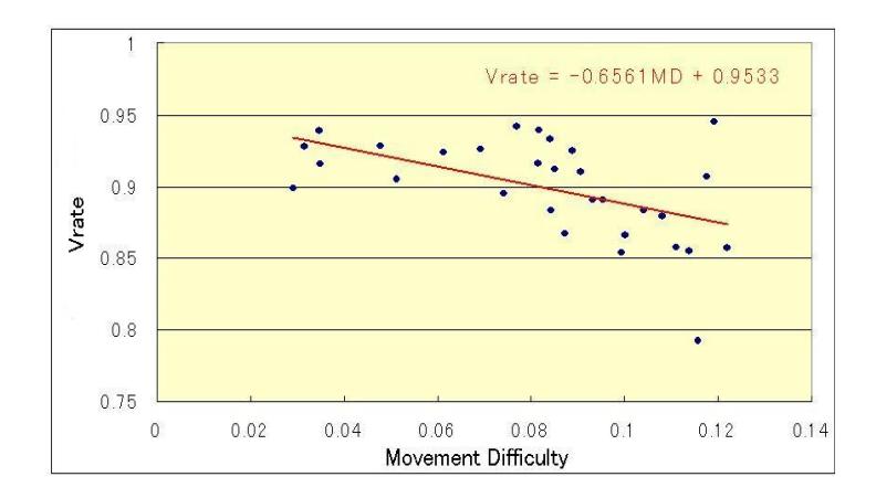
We analyze the dependency relationship between the difficulty of movement and score of RoboCupRescue ($rescue\ score$). We use the ratio of the resuce score ($\frac{simulation\ score}{initial\ score}$).

We use regression analysis and develop the following expression and figure 1.

$$V_{rate} = -0.3164 \mathbf{MD} + 0.8999$$

$V_{rate}$: estimation of the rate of rescue score

$MD$: Movement Difficulty

Thus there is a relation between the $movement\ difficulty$ and the rescue score. We analyze the relationship for more agent algorithms(strategies), and change the strategies in the simulation. The agent chooses the optimal strategies for any maps in this way.

Fig. 1. Dependencity Relation Between Rescue Score and Movement Difficulty

4 Conclusion

First, we defined eleven definitions and sixteen parameters for the complexity of road network.

Second, we developed the $movement\ difficulty$ from the complexity of the road network. The $movement\ difficulty$ is expressed with eight parameters of complexity for road network.

Third, we analyzed the dependency relationship between the $movement\ difficulty$ and the score from the RoboCupRescue simulation. Finally, we developed the estimation of the rate of the rescue score. Thus agents can choose appropriate algorithms for any maps by analyzing them.

Future tasks include analyzing more algorithms and developing the agents so that they can choose optimal strategies from various algorithms.

References

Kinoshita, T., Sugawara, K.: Agent Oriented Computing ~ Foundation and Application of Agents ~ in Japanese. Soft Research Center (1995)
Kazunori I., Nobuhiro I., Youhei K., Naohiro I.: Complexity of Road Networks as Agents' Environments Second KES International Symposium on Agent and Multi-Agent Systems: Technologies and Applications(KES-AMSTA) (2008) 474–484
V.Pynadath, D., Tambe, M.: Multiagent teamwork: Analyzing the optimality and complexity key theor ies and models. Proceedings of International Joint Conference on Autonomous Agents and Multi-Agent Systems(AAMAS) (2002) 873–880
Asano, T., Iwano, K., Umeo, H., Yamashita, M., Wada, K.: Algorithm Introduction in Japanese. Volume 1. Kidai Kagaku sha Co., Ltd (1995)
Asano, T., Iwano, K., Umeo, H., Yamashita, M., Wada, K.: Algorithm Introduction in Japanese. Volume 2. Kidai Kagaku sha Co., Ltd (1995)
Harary, F.: Graph Theory: New Ed edition. Westview Press (1994)
Wikipedia: Flow network. http://en.wikipedia.org/wiki/Flow_network (2007)