RoboCupRescue2010 - RescueSimulationLeague TeamDescription < NAITO-Rescue >
Toshihito Suzuki, Nobuhiro Ito
Department of Electrical and Computer Engineering, Nagoya Institute of Technology
Abstract Disaster simulation is one of the approaches for reducing disaster damage. The RoboCupRescue simulation package is one of the most popular simulation packages for this purpose. In this paper, we describe the NAITO-Rescue RoboCupRescue team simulation system. It is known that RoboCupRescue Agents are affected by the environment and thus we developed the system with a scientific approach to predict the RoboCupRescue score establishing the relationship between the simulation agents and the environment. In particular, we focused on the " building information " simulation segment of the environment in addition to " road network " that has been our focus in recent work.
Introduction
The RoboCupRescue(RCR) simulation package is a disaster simulation system in which three types of disaster relief teams, the fire brigade, the ambulance team and the police force act to reduce the disaster damage resulting from earthquakes in a " map " of the environment. RCR agents are affected by this map. For example, agent A1 can work better than agent A2 in an environment E1, and agent A2 can work better than agent A1 in an environment E2. Such a scenario is common in RCR simulations. Thus it is necessary to analyze the dependency relationship between the map and the RoboCupRescue score. In our recent work, the RCR score was affected significantly by the road network. However, It was not enough to predict the RCR score. This paper increases the accuracy of prediction using building information when analyzing the dependency relationship. Finally, we developed agents that can choose the optimal algorithm for several maps.
The Agent's Environment
In this section, we analyze a map as the RCR agent 's environment. In general, map data includes features such as roads, railroads, rivers, buildings, geographical features and so on. In the RCR simulation, the map includes only roads and buildings. We focused on building information and road networks to analyze the dependency relationship between the map and the RCR score. There are five components to the map data, namely the building area, the building property, the position relationship of the building, the position relationship of the building and roads, and the density that affects disaster-relief work. In this paper, we quantify building information and road networks for each of the components, and define them as indexes of buildings and roads. We define each index in 2.1.
Indexes of buildings and roads
In this section, We define Indexes of buildings and roads. Semi gross building coverage is the feature relates to building area. Contour length is the feature relates to building property. Degree of dependence and distance to adjacent buildings and dispersal of buildings are the features relate to position relation of building. length of adjacent road and interspace ratio are the features relate to position relation of building and road. total road length and road density and building density are the features relate to density.
semi gross building coverage
First, we calculate the building coverage for each gross area on the maps. Next, we calculate the average of building coverage for all semi-gross areas. We define this average as the index of building coverage for each semi-gross area on a map. Gross area means a land area identified by the center lines of surrounding roads and a semi-gross area is derived from the gross area by the loss of the road areas.
contour length
We calculate the average of the circumference of the buildings and define this average as the index of contour length in the map.
degree of dependence
The degree of dependence is the ratio of a building area to the largest building area among adjacent buildings. We calculate the degree of dependence of each building, and average all degrees of dependence. We define this average as the index of the degree of dependence on a map.
distance to adjacent buildings
We calculate the distance to the farthest building among the adjacent buildings, for each building. Then we calculate an average of the distances. We define this average as the index of distances to adjacent buildings on a map.
dispersal of buildings
For each building on a map, we calculate the difference between the minimum distance to the nearest building and the maximum distance to the farthest building among adjacent buildings. Then we calculate an average of this difference. We define this average as the index of the dispersal of buildings on a map.
length of adjacent road
We calculate the distance to the nearest road for each building on a map. Then we calculate the average of this distance. We define this average as the index of the length of adjacent roads on a map.
interspace ratio
We measure the length of building verges to the nearest road and the nearest road length for each building on a map. Then we calculate the length of building verges to the nearest road, divided by the nearest road length. We call this ratio the inter-space ratio of the building. Then we calculate an average of the inter-space ratio of all the buildings on a map. We define this average as the index of the inter-space ratio on a map.
total road length
We define the total road lengths on a map as the index of the total road length.
road density
Road density is a ratio of the area of road to the area of the map. We define this ratio as the index of the road density on a map.
building density
The building density is the ratio of the number of buildings on a map to the area of the map.
Analysis and Prediction
We specified the relationship between an agent and the indexes defined in 2.1 to predict the agent 's score. We simulated RCR on 24 maps of Japanese cities. The agents used are the agents of the MRL team, the Impossibles08 team, the SUNTORI team and the CSU Yunlu team. We analyzed the relationship between the indexes and the RCR score with regression analysis.
Regression analysis
We obtain the following prediction formula for each agent. Formula (1) is calculated for the MRL team, Formula (2) is calculated for the Impossibles08 team, Formula (3) is calculated for the SUNTORI team, and Formula (4) is calculated for the CSU YunLu team.
$V_{rate}$ is the ratio of RCR score after simulation finished to RCR score before simulation started. We henceforth use $V_{rate}$ as a RCR score.
$$V_{rate1} = (-3.16e^{-2} \times c_1 + 8.17e^{-5} \times c_2 + -2.98e^{-3} \times c_3 + 1.08e^{-3} \times c_4 + 9.00e^{-2} \times c_5 + -2.30e^{-4} \times c_6 + -8.94e^{-2} \times c_7 + -2.84e^{-7} \times c_8 + -4.59e^{-2} \times c_9 + -15.7 \times c_{10} + 0.929)/S_{start}$$
(1)
$$V_{rate2} = (-1.21e^{-2} \times c_1 + -1.90e^{-3} \times c_2 + 6.30e^{-3} \times c_3 + 1.12e^{-2} \times c_4 + 1.93e^{-1} \times c_5 + -2.85e^{-7} \times c_6 + 1.00e^{-2} \times c_7 + -2.85e^{-7} \times c_8 + -1.70e^{-1} \times c_9 + -9.30 \times c_{10} + 0.836)/S_{start}$$
(2)
$$V_{rate3} = (-2.93e^{-2} \times c_1 + -7.16e^{-5} \times c_2 + 4.22e^{-3} \times c_3 + 1.37e^{-2} \times c_4 + 2.02e^{-1} \times c_5 + -2.45e^{-3} \times c_6 + 5.19e^{-2} \times c_7 + -1.50e^{-6} \times c_8 + 3.90e^{-3} \times c_9 + 14.8 \times c_{10} + 0.653)/S_{start}$$
(3)
$$V_{rate4} = (9.80e^{-3} \times c_1 + 2.80e^{-4} \times c_2 + -4.60e^{-3} \times c_3 + -2.79e^{-3} \times c_4 + 7.77e^{-2} \times c_5 + -4.30e^{-4} \times c_6 + 2.50e^{-2} \times c_7 + -2.75e^{-7} \times c_8 + -2.60e^{-3} \times c_9 + -20.1 \times c_{10} + 0.839)/S_{start}$$
(4)
$V_{rate}$: estimation of the rate of rescue score
$S_{start}$: The RCR score before simulation started
c1: Semi gross building coverage
c2: Contour length
c3: Degree of dependence
c4: Distance to adjacent building
c5: Dispersal of buildings
c6: Length of adjacent road
c7: Total road length
c8: Interspace ratio
c9: Road density
c10: Building density
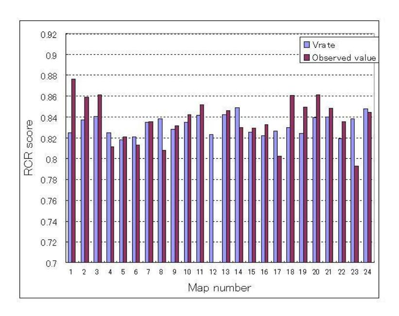
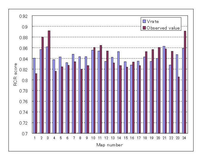
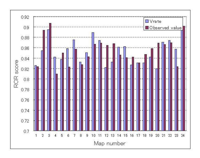
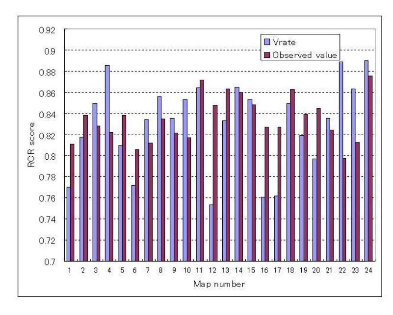
In the formula, the coefficient of each of the indexes means the degree of efficiency for the indexes that affects the RCR score. We can learn which component of the map data affects an agent 's actions from these formulae. Next, we predict the RCR score using previous formulae and map data. Then we compare the prediction score and the observed score. Figs. 1, 2, 3 and 4 show the comparisons for each of the 4 agents 'algorithms. In the figures, the x-axis label defines the number of maps using the simulation. The lack of a graph of map number 12 in figure 4 means the agent cannot take any action on the map because of any error. The prediction accuracy seems adequate from these figures.
Prediction of RCR score
We considered using the prediction of the RCR score to improve our team agent's performance. First, We set up a number of algorithms that obtained good scores in the previous RoboCupRescue competition. This was easy because the first division agents 's algorithms are not secure. Next we calculated indexes of buildings and roads before starting the dynamic simulation. Then we calculated the prediction score for each of the agents that were set up. From this we selected the optimal agent algorithm for any of the maps. For example, if in simulating with map number 3 in figures 1-4, the Impossibles08 had the best prediction score, we changed the algorithm to the Impossibles08. On the other hand, if in simulating with map number 4, the SUNTORI had the best prediction score so we choose the SUNTORI algorithm.
Conclusion
First, we defined 10 indexes of buildings and roads. Second, we analyzed the RCR scores and defined indexes for various agent algorithms to analyze the relationship between the score and the map. Finally, we predicted the RCR score of the agent from the results of the analysis. Then we selected the most appropriate algorithm for each of the various maps.