Team Description Paper SBCe_Saviour Virtual Robots League-2009

Eslam Nazemi, Ashkan Radmand, Amir Saman Memaripour, Iman Sarrafi, Mohammad Hossein Sedighi Gilani, Reza Bakhshi

Shahid Beheshti University, Tehran, Iran

Abstract The main approach of our team is to avoid using grid based mapping and to use a vector based mapping instead. According to that, a fast vector based SLAM, and a vector based navigation system were designed and implemented. Although this approach needed so many new methods to be designed and perfected, we had achievements such as less memory usage, less communication in map, and more precise values. The main sensor used in our agent is the Sick-LMS sensor, which is the only sensor our SLAM uses.

Keywords: Virtual Robots, Mobile Robots, SLAM

1 Introduction

Recently, all the virtual robot's agents are designed using grid based maps. Even the standard output for the competitions is a Geotiff file. The main reason they are so popular is that they are easy to use; specially in determining the similarity of maps any image based similarity method can be used (e.g. cross-correlation of two images). But these grid based maps, have 4 drawbacks:

• 1. A resolution has to be defined.
• 2. If the resolution is too low, the resulted can't be used. (the map will be low detailed)
• 3. If the resolution is too high, the running time of a simple cross-correlation may exceed the operational limit.
• 4. The maps will be big in the size, so sending and receiving maps will fill the wireless bandwidth.

Because of the reasons above, we tried to use a vector based map instead of the usual grids. In order to do that, we needed a new SLAM and a navigation method.

In section 2 the structure of the vector map and the way that the sensors output is converted to this kind of map, are described; section 3 describes the SLAM we implemented for such a map. Sections 4 and 5 describe how the communication and the navigation is handled by the agents. And section 6 concludes the paper.

2 The Map Structure

In order to start with a simple structure which can show almost all possible maps, our vector map is designed of one type of vector, the "Line Type Vector".

This vector type is used to store the identified line segments of the walls. So they will need to store two points as the start and the end of the line segment. But because the sensors are noisy, and these maps have to somehow get fused with each other, there are three more attributes. First is the ppl value, that stands for the "points per line", which is the logarithm of the number of points found on that line over the number of times that line is seen. The second is the standard deviation of the line; the points that have made the line were not precisely on that line. And the third is the number of times that line has been seen, which is needed to calculate the ppl value.

So the structure can be defined as below:

Fig. 1 definition of the line segment vector

After defining the structure, we have to define a method that converts the laser's output, to an array of defined vectors. To do so, the following series is done:

• 1. Each distance should be converted into its correspondent point.
• 2. An O(n) algorithm is used which clusters the points into clusters that more likely belong to the same line.
• 3. The fittest line algorithm is used over each cluster.
• 4. The first node of the cluster is selected and its projection over the fittest line is assumed to be the "a" value.
• 5. The last node of the cluster is selected and its projection over the fittest line is assumed to be the "b" value.
• 6. The "seen" value is equal to 1.
• 7. The "ppl" value is the logarithm of the size of the cluster. (because "seen" equals 1)
• 8. The standard deviation of the distances of the original points to the line is calculated as "sigma".

Now a local vector based map is generated out of the laser output, which is the list of line vectors.

3 SLAM

Any SLAM method has two steps. The first step is to calculate the transition vector, and the second step is to build up a global map using the local maps and their transitional vectors.

3.1 Transition Vector

In order to calculate the transition vector, first the rotation is calculated, then assuming the robot has first rotated and then moved forward, the movement vector is calculated.

3.1.1 Rotation

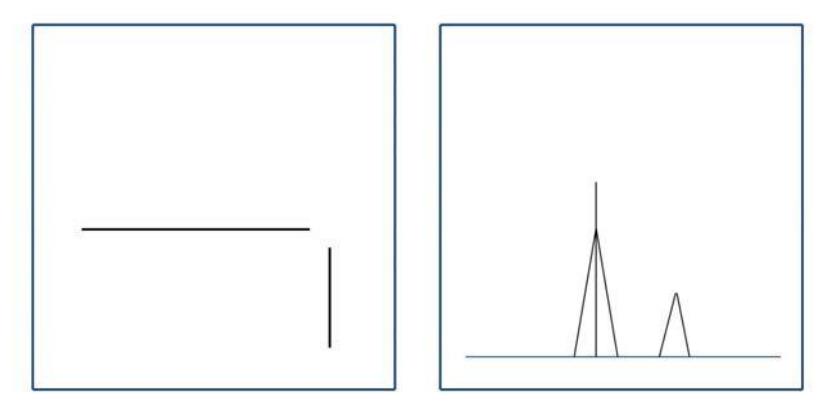
To calculate the rotation value, a histogram is generated. In this histogram, each line is represented by a Triangular function. Fig 2 shows a sample of a two lined map converted to this histogram.

Having two histograms (local map and the pre local map), they are convolved into each other. The angle that has the most convolution value is the angle of Rotation.

Fig. 2 Left image, is a simple two lined map. Right image is the theta histogram of the map. The triangles are placed at 0 and π/2 values. The height of each triangle is equal to the ppl value and the wideness of each is defined using the sigma value.

3.1.2 Movement

After calculating the "θ" value, the current local map's vectors are rotated by a simple 2x2 rotation matrix, so that the rotated current map and the previous map's line segments are almost parallel.

$$\begin{bmatrix} new_{-}x \ new_{-}y \end{bmatrix} = \begin{bmatrix} \cos\theta & -\sin\theta \ \sin\theta & \cos\theta \end{bmatrix} \begin{bmatrix} x \ y \end{bmatrix}$$

After rotating the map, we need some candidates for transition vector and a method to find out which one of the candidates is the best one that fits the two maps. To define such a fitness function, we defined a fitness function which implies on two line segments. The function is defined as below:

$$F(v_{1}, v_{2}) = \frac{P(v_{1}, v_{2}) ppl_{1} \cdot ppl_{2}}{d(v_{1}, v_{2}) + 1}$$

Where,

$$P(v_{1}, v_{2}) = \begin{cases} 1 & teta_dif(v_{1}, v_{2}) \le 3\ .5 & 3 < teta_dif(v_{1}, v_{2}) < 5\ 0 & otherwise \end{cases}$$

And "d" is the Euclidian distance of the line segment joining the middles of two vectors.

After defining the fitness function for line segments, we defined the overall fitness function as follow:

Fig.3 Fitness function used to calculate the fitness of two vector based maps

To generate the candidates, the easiest method is to use a genetic algorithm, which somehow generates these candidates using the previous generation. But we used a combination of a geometric method and the hill climbing algorithm.

At first, each line's conjunction with its neighbor line is calculated. This gives us some points which we call junction points. Then each junction point in pre-local map is linked to each junction point in local map and the resulted vectors are categorized according to their length and orientation. The top 10 vectors are selected, and the fitness function is calculated over them. The vector with the greatest fitness value is selected as the first step movement vector.

In step two, an iterative algorithm is used to refine the first step vector. To do so, a small distance is selected and the four neighbors with that distance of the vector are generated. If none of them had a better fitness value, the distance is dividend by 2 and the same is done, otherwise the vector with the best fitness is selected and the iteration continues.

3.2 Building a Global Map

In order to build a global map, a fuzzy method is designed and used. The fuzzy membership value of each line is calculated according to the ppl and sigma value. Then the lines with the maximum similarity which is calculated using the fuzzy membership value, length, start point, end point and the orientation of the line, are fused to each other and they are replaced by a new set of start point, end point, ppl, sigma and seen.

4 Communication

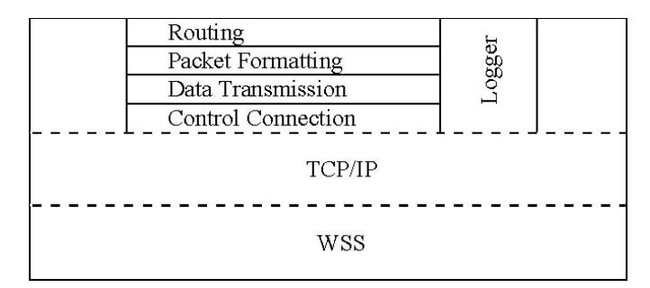
Regarding the high importance of communication among agents and its key role in efficiency of the team's output, this is one of the most important parts of the project. Figure below illustrates the general structure of our Communication System.

Fig.4 structure of the designed Communication System

Components of this figure are described in the following:

1. Control Connection Layer

This layer makes the lowest layer of our structure and is responsible for managing the control connection with WSS via TCP/IP protocol. We have functions implemented for operations such as Get Signal Strength, Initial Robot, Reverse DNS and DNS. The scope of this layer is limited to sending and receiving control instructions to/from WSS.

2. Data Transmission Layer

The bases of sending and receiving information between two agents are prepared in this layer. Send Data, Receive Data and Buffer Data are some functions implemented in this section. What made us separate this layer from the Control Connection Layer was the difficulties of implementation and debugging these two sections together in one unified class?

3. Packet Formatting Layer

Packet Formatting is the other layer included in our structure concerning the virtual league world cup. In this layer, we have functions for formatting information, compressing them if needed, and detection and correction of errors. Information formatting is necessary because of the variety of data types transferred among agents, as each data type demands its own interpretation and decision making methods. Image, text, and communication instructions could be recalled among these data types. By the other hand, the need to faster data transfer and shorter connection time between agents shows the necessity of data compression, for which compressing algorithms have been used. Also, concerning the environmental noises and the high importance of bandwidth between two agents, error detection and error correction techniques have been included in this layer [1, 4].

4. Routing Layer

This layer is included in our structure for two main reasons:

• I. Finding the best communication path, this is considered the path with least possible noises and intermediate agents.
• II. The need to a connected graph which provides a communication path between any two agents.

In order to achieve the above goals, Dijekstra's shortest path algorithm [2] was chosen among possible solutions. In our system, after the communication between each two agents is started each of them sends its signal strength with other agents to the other side in form of a package. This transferred information is used by each side for updating the complete communication graph it has. This graph helps making decisions about the data transfer path. Each agent along this path will work as a communication bridge that only gets and passes the data [3].

5. Logger

This layer is only used for controlling the behavior and working details of the structure.

5 Navigation

For navigating, we used a method similar to the potential field. The main difference is that potential fields are usually generated in a grid map, which we don't have in our agents. In order to navigate, first we defined forces on the following candidates:

• 1. Each line segment (wall) has a repelling force.
• 2. Robots also repel each other.
• 3. If there is an aim for robots, each aim attracts robots.
• 4. Every 15 seconds, each robots current position becomes a permanent repelling force.
• 5. An accessibility value is calculated by using the signal strength and the placements of the robots, this value is also assumed to be a force.

Using these five forces, in each state a robot can do the following actions:

• 1. Reducing (increasing) left wheel's velocity by 1.
• 2. Reducing (increasing) right wheel's velocity by 1.

These actions may make at most 9 different actions which the robot can do in one step. Knowing the position and velocity, we can almost predict the 9 actions' results. So for those 9 positions, the potential is calculated and the best action is selected to be done. If more than one step ahead is calculated, the navigation will be less faulty.

6 Conclusion

The system has not been fully tested, but by the partial tests the results are good. Hopefully the system is completed until IranOpen competition. This kind of map, describes the circles and curves as fragmented line segments. Curves and circles are not usually used in buildings or the usual shaped objects, but it's better to add curve vector to the vectors used in the map. But that makes the SLAM and the navigation potential forces more complex.

References

1. Morelos-Zaragoza, R.H.: The Art of Error Correction Coding (2nd ed.) Wiley. (2006)
2. Cormen, T.H., Leiserson, C.E., Rivest, R.L., Stein, C.: Introduction to algorithms (2nd ed.) Mc Graw Hill. (2001)
3. Doyle, J.: Routing TCP/IP Volume I (1st ed.) Cisco Press. (1998)
4. Razavi, R., Fleury, M., Ghanbari, M., Sadeghzadeh, M.: Delay-aware interleaving and forward-error correction for video over wireless: a bluetooth case study, ACM. (2007)