Tech United Eindhoven RoboCup Adult Size Humanoid Team Description 2013

P.W.M. van Zutven, T.M. Assman, J. Caarls, C. Çilli, T.P.M. Boshoven, E. Ilhan, J.A.J. Baelemans, D.J.F. Heck, M.P.A. Spoelstra, H. Nijmeijer

Eindhoven University of Technology, Department of Mechanical Engineering, Dynamics and Control Group, Den Dolech 2, P.O. Box 513, 5600 MB Eindhoven, The Netherlands

www.techunited.nl

Abstract This document presents the 2013 Tech United Eindhoven adult size humanoid robot team from The Netherlands. In this description paper we present the model, parameter estimation and simulator of our humanoid robot TUlip. We introduce the walking gait and contribute a feedback controller with feedforward dynamics compensation and iterative learning control. We describe the vision system, localization and world model, which are used during the humanoid robot soccer games at the RoboCup 2013 in Eindhoven, the Netherlands. Finally, we contribute a new simulator of TUlip including a RoboCup scenario implemented as Robot Operating System (ROS) package in Gazebo.

1 Introduction

Since five years, the humanoid robotics team from the Eindhoven University of Technolgy has participated in the annual RoboCup adult size humanoid league as part of Tech United. In this document we introduce our humanoid robot TUlip, which is intended for competitions in the adult-size humanoid league at the RoboCup 2013 in Eindhoven, the Netherlands. This paper describes the current state of the robot, its model and the model parameter estimation method [8]. We contribute a gait design method using the linear inverted pendulum model [2] and an enhanced controller structure with joint feedback control, feedforward dynamics compensation and iterative learning control. Moreover, we present an improved vision, localization and world model and contribute our new robot simulator including RoboCup field scenario, which is implemented as Robot Operating System (ROS) package in Gazebo.

Tech United Eindhoven commits to participate in RoboCup 2013 in Eindhoven and to provide a referee with sufficient knowledge of the rules of the Humanoid League. We do not use software from other teams, and we contribute to the community with our simulator which is available as open source. Over the years, research on TUlip has resulted in several scientific publications: [1, 7–10]. The paper is organized as follows. In Section 2 we introduce our humanoid robot TUlip, including its model, parameter estimation and simulator. In Section 3 we explain our walking algorithm. In Section 4 we describe our software architecture that includes vision localization, world model and strategy.

2 TUlip hardware, model and simulator

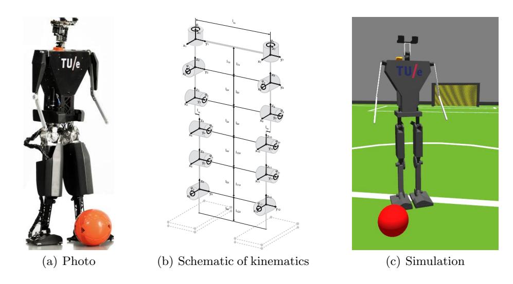
TUlip is a 125 cm tall, 23 kg heavy, anthropomorphic adult-size humanoid robot as depicted in Fig. 1(a). Advanced hardware specifications can be found on our website [5] and in previous RoboCup papers [11]. Kinematically, we model TUlip as a chain of rigid bodies. As schematically depicted in Fig. 1(b), the kinematic model has six revolute joints in each leg. The dynamic equations of motion can be derived using Euler-Lagrange methods:

$$D_j(q)\ddot{q} + C_j(q,\dot{q})\dot{q} + G_j(q) = \tau, \tag{1}$$

where $q \in \mathbb{T}^{12}$ is the state vector, $D_j \in \mathbb{R}^{12 \times 12}$ is the symmetric positive definite inertia matrix, $C_j \dot{q} \in \mathbb{R}^{12}$ is the vector of Coriolis and centrifugal terms, $G_j \in \mathbb{R}^{12}$ is the gravity vector and $\tau \in \mathbb{R}^{12}$ are the joint torques. The index $s \in {R, L}$ indicates whether (1) is derived with the base coordinate frame in the right (R) or left (L) foot.

The lengths of the links of the biped are measured on the real robot. The masses, inertias and positions of the centers of mass of each link are estimated in several identification experiments [8] as follows. We define the center of mass (CoM) position normal to the coronal, sagittal and transverse plane as $x_c$, $y_c$ and $z_c$ respectively. To estimate the model parameters in these equations the center of pressure (CoP) is measured for a number of static postures of the robot. The CoM position equations are rewritten to a so-called base regressor form to fit the model parameters to the measurement data:

$$\left[x_c \ y_c \ z_c\right]^{\top} = R_b(q)\vartheta_b,\tag{2}$$

where $R_b(q)$ is the regressor matrix and $\vartheta_b$ is a vector of base parameters. The base parameters are combinations of parameters such that the columns of the regressor matrix are linearly independent. The measured CoP position is equal to the CoM position projected onto the ground. Therefore only the equations in $x_c$ and $y_c$ direction can be used to identify the base parameter set $\vartheta_b$. The equation for $z_c$ however contains the same parameter combinations. This means that not all parameters can be estimated independently and thus that the estimated parameters $\vartheta_b$ are only useful when used in the equations for the CoM position. We use these equations in the design of the gait and in the controller as is explained in Section 3. We are also planning to perform dynamic experiments and fit model parameters in the equations of the Zero Moment Point (ZMP) position to experimental data of the CoP.

Application of model (1) is twofold. Firstly, it is used in gait design and in the controller, which is explained in Section 3. Secondly, we implemented this model in the Gazebo simulator to simulate the walking trajectories and validate the performance of the controllers. A simulator improves safety of the robot and its environment and, additionally, we can test high-level strategies faster and, if necessary, under ideal conditions. Gazebo has been chosen because it is an open source, fast simulator that uses the Open Dynamics Engine and it is integrated in the Robot Operating System (ROS). Moreover, Gazebo features appealing visualizations (Fig. 1(c)), so that the vision module can be simulated as well. A modeled ball and soccer field even allow for testing the ball tracking and localization algorithm, respectively. The model itself (including the ball and field) is available on-line to support other teams [6], together with a validation study of the simulation model using experiments [1].

3 Balance, gait design and control

Balance of humanoid robots consists of finding and controlling joint motions such that the robot can walk without falling. In this section we describe the gait design, trajectory generation and control of TUlip. On TUlip, we use dynamically stable gaits. A dynamically stable gait is a gait designed such that the robot is always in dynamic balance, i.e. the robot always has its zero moment point (ZMP) within the support polygon of its feet.

The design of the dynamically stable gait consists of two parts. First, we describe how the preferred CoM and swing foot trajectories are designed in task space and secondly how these task space trajectories are mapped to joint trajectories using an inverse kinematics algorithm. Finally, we describe the controller that computes the joint torques to follow the desired gait.

3.1 Gait design

In this section we explain the design of a dynamically stable gait for TUlip. A gait consists of multiple steps $k \in {1, . . . , n}$. In each step we prescribe the desired task space CoM position, torso orientation and swing foot position and orientation with respect to the stance foot.

The positions of the CoM and swing foot are prescribed by the evolution of a linear inverted pendulum [2]. The evolution of the horizontal dynamics in $x_c$ and $y_c$ direction in a plane at height $z_c$ for $h \in {x_c, y_c}$ is:

$$h_{c,k}(t) = h_{c,k}(0) \cosh\left(\frac{t - t_{0,k}}{T_c}\right) + T_c \dot{h}{c,k}(0) \sinh\left(\frac{t - t{0,k}}{T_c}\right), \quad T_c = \sqrt{\frac{z_c}{g}}, \quad (3)$$

where $t_{0,k}$ is the time at the beginning of step $k$. The total desired position of step $k$ yields:

$$p_{d,k} = \left[ x_{c,k} \ y_{c,k} \ z_c \ 2x_{c,k} \ 2y_{c,k} \ \text{sat}(z_c - |v_f x_{c,k}|, h_f) \right]^\top, \tag{4}$$

where the swing foot position mirrors the CoM position to achieve a symmetric step. The parameters $h_f$ and $v_f$ define the height and vertical velocity of the swing foot respectively.

The orientations of the torso and swing foot are always straight up and parallel to the ground respectively, and in the desired walking direction. They are both parametrized in the vector $\varphi_d$ by three angles using the roll-pitch-yaw convention.

Finally, the task space trajectories of step $k$ are defined as $x_{d,k} = \left[ p_{d,k}^T \ \varphi_d^T \right]^T$ and stitching multiple steps together yields the desired task space trajectories for the entire gait: $x_d = x_{d,1} ... x_{d,n}$. Besides the trajectories based on the linear inverted pendulum model, we separately define trajectories for kicking using cosine velocity profiles [11].

3.2 Inverse kinematics

The task space trajectories defined in the previous section can be mapped to joint angles in order to control the robot in joint space. We use an inverse kinematics algorithm based on differential kinematics:

$$\dot{x}_d = J(q_d)\dot{q}_d,\tag{5}$$

where $J \in \mathbb{R}^{12 \times 12}$ represents the geometric Jacobian of the CoM position, torso orientation and swing foot position and orientation with respect to the stance foot and $\dot{q}_d \in \mathbb{R}^{12}$ are the desired joint angular velocities, which are given by:

$$\dot{q}_d = J^{-1}(q_d)\dot{x}_d,\tag{6}$$

such that the desired joint angles $q_d \in \mathbb{T}^{12}$ are given by:

$$q_d(t) = \int_0^t \dot{q}_d(\varsigma) d\varsigma + q_d(0). \tag{7}$$

But, on a physical robot this must be implemented in discrete time and discrete integration may lead to drift. Therefore, we use an inverse kinematics algorithm proposed in [3]. Hereto, we define the error between the desired and (possibly drifted) computed task space position as:

$$e_p = p_d - p_e, \tag{8}$$

where $p_e$ is the computed task space position of the CoM and swing foot using forward kinematics of the desired joint angles $q_d$. For the orientation we derive the desired roll-pitch-yaw rotation matrix $R_d = \left[ n_d \ s_d \ a_d \right]$ from the desired task space orientation $\varphi_d$ where $n_d$, $s_d$ and $a_d$ are simply the columns of $R_d$. Similarly, the roll-pitch-yaw rotation matrix computed by forward kinematics of the desired joint angles $q_d$ is $R_e = \left[ n_e \ s_e \ a_e \right]$, which results in the task space orientation error:

$$e_o = \frac{1}{2}(n_e \times n_d + s_e \times s_d + a_e \times a_d). \tag{9}$$

These errors (8) and (9) are used in (6) to compensate for drift:

$$\dot{q}_d = J^{-1}(q) \begin{bmatrix} \dot{p} + K_p e_p \ L^{-1}(L^{\top} \omega_d + K_o e_o) \end{bmatrix}, \tag{10}$$

where

$$L = -\frac{1}{2}(S(n_d)S(n_e) + S(s_d)S(s_e) + S(a_d)S(a_e)), \tag{11}$$

with $S(\cdot)$ the skew-symmetric matrix of its vector argument. The system (10) is asymptotically stable for the positive definite matrices $K_p = \text{diag}(K_{p,1}, . . . , K_{p,6})$ and $K_o = \text{diag}(K_{o,1}, . . . , K_{o,6})$. Moreover, it can be shown that discrete time integration of (10) in (7) does not result in drift [3].

3.3 Control

The predefined joint trajectories need to be tracked on the humanoid robot such that it performs the desired gait. We implemented a controller consisting of three parts: a local joint PD feedback controller ($\tau_{fb}$), a model based dynamics compensation feedforward controller ($\tau_{ff}$) and an iterative learning controller ($\tau_{ILC}$):

$$\tau = \tau_{fb} + \tau_{ff} + \tau_{ILC}. \tag{12}$$

Feedback control We use local PD control on each joint to track the desired reference trajectories and to make the system (1) robust against disturbances:

$$\tau_{fb} = K_P e + K_D \dot{e},\tag{13}$$

where $\tau_{fb}$ are joint controller feedback torques, $e = q_d − q$ are the tracking errors and $K_P = \text{diag}(K_{P,1}, . . . , K_{P,12})$ and $K_D = \text{diag}(K_{D,1}, . . . , K_{D,12})$ are the controller gains. These gains are tuned for maximal performance without destabilizing the system.

Feedforward control Due to the limited bandwidth of the local PD controllers, there are always feedback tracking errors in the joint angles. As a solution, we implemented a model based feedforward algorithm on TUlip to improve the tracking performance. The feedforward torques are computed from (1):

$$\tau_{ff,j} = D_j(q_d)\ddot{q}_d + C_j(q_d, \dot{q}_d)\dot{q}_d + G_j(q_d) := \tau_d + \tau_c + \tau_q. \tag{14}$$

The dynamics compensation torques $\tau_{ff}$ are computed using a similar heuristic approach as in [2] for single support as well as double support. The approach is based on the ratio $\alpha$ between the distances from the CoM of the biped to its right ($\alpha = 1$) and left foot ($\alpha = 0$) respectively. The gravity compensation is now given by:

$$\tau_{ff} = \alpha \tau_{ff,R} + (1 - \alpha) \tau_{ff,L},\tag{15}$$

where $\tau_{ff,R}$ and $\tau_{ff,L}$ are the gravity vectors computed in (14) with the base coordinate frame in the right, respectively the left foot. This approach automatically works in single and double support due to the parameter $\alpha$.

Because gravity compensation $\tau_g$ showed significant control improvement during RoboCup 2012, we are currently investigating additional feedforward control of the inertial terms $\tau_d$ and Coriolis terms $\tau_c$ for RoboCup 2013. The desired joint velocities $\dot{q}_d$ follow directly from the inverse kinematics algorithm (10). The desired joint accelerations $\ddot{q}_d$ are obtained by numerical differentiation of $\dot{q}_d$.

Iterative learning control For RoboCup 2013, we are also investigating the use of Iterative Learning Control (ILC) to learn a feedforward control action $\tau_{ILC}$ based on previous experience. The application of the adaptive ILC, designed in [4] to control a single manipulator, is currently investigated. The control action of step $k$ for joint $i \in {1, ..., 12}$ to control the joint angle $q_i$ is computed as

$$\tau_{ILC_{b,i}} = \eta(\dot{e}{k,i})\theta{k,i}(t),\tag{16}$$

with

$$\eta(\dot{e}{k,i}) = \left[ \dot{e}{k,i} , \tanh(\beta \dot{e}_{k,i}) \right],\tag{17}$$

$$\theta_{k,i}(t) = \theta_{k-1,i}(t) + \Gamma_i \eta^T (\dot{e}{k,i}) \dot{e}{k,i}(t), \tag{18}$$

where $\theta_{1,i}(t) = 0$. The gain $\beta > 0$ should be chosen sufficiently large to approach a sign function. The gain matrix $\Gamma_i \in \mathbb{R}^{2 \times 2}$ is tuned to trade-off convergence with robustness.

4 Vision, Localization, World Model and Strategy

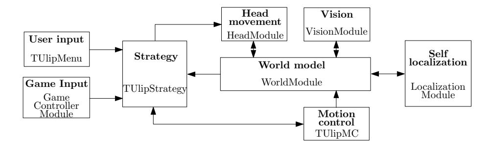
An architectural redesign was done, in order to make TUlip's software more component-based. The reason for this is the addition to more higher-level components, such as strategy. This way, it is easier to replace software components and connect new components to the existing architecture. The new architecture is data-driven by nature. The software architecture currently consists of the following eight components, shown in Fig. 2:

Vision does image processing to subtract features from the images produced by the cameras. Interesting features in a RoboCup game are ball, goals, opponents, lines and field markers. The vision software proceeds basically in three steps: 1) segment by color, 2) detect features in segmented image and 3) apply inverse model of the lens to calculate 2D angle to each feature. Vision can only provide position of the object on a picture that it has captured. All information from Vision is relative to the robot and is subject to observation noise.

World model and Localization interpret Vision outputs. Objects which do not change position, e.g. field lines or goals, are used for robot localization. Dead reckoning information is used to estimate robot position when there is no vision information available. Knowing the robot position, other objects which move, e.g. opponent or ball, can be localized on the field. Localization and world modeling are done by Extended Kalman Filters (EKF). One EKF is used for robot localization. Having robot dead-reckoning information and robot's observations about the field, EKF estimates robot position and its uncertainty. As long as the robot sees some distinct features of the field, it gains confidence about its position estimate, otherwise it becomes uncertain. Knowledge of the robot position helps interpreting positions and motions of other objects on the field. An EKF is used for each movable object, namely the opponent and the ball. EKF's are designed and tuned in such a way that they can track moving objects, even if the motion is not caused by robot's actions.

Head movement controls the position of the head, making the robot look around or concentrate on a specified position.

Motion control controls the robot's legs. In addition to this, it provides detailed information about the legs for real-time visualization and analysis.

Game input provides information retrieved from referee software, in order to keep track of game progress.

Strategy combines all inputs in order to decide what should be done, the strategy for the dribble and kick challenge can be found in [11].

User input provides an interface for controlling the strategy. Currently, this component is implemented in the form of a small menu.

The architecture is easily extendable by additional components. For example, a connection was made between the Motion control component and Matlab, to allow for real-time analysis of the robot's movements. In addition, the simulator of TUlip in Gazebo can be connected to this component, in order to test the robot's movement before executing it on the real system.

5 Conclusion

In this document we presented the Tech United Eindhoven adult size humanoid robot TUlip. We described its model, parameter estimation and simulator. Moreover, we explained the gait design and trajectory generation for dynamically stable walking and contributed the local joint feedback control, feedforward dynamics compensation and iterative learning control. Finally, we described TUlip's software components: vision system, self localization, world model and strategy.

References

1. T. Assman, P.W.M. van Zutven, and H. Nijmeijer. Qualitative validation of humanoid robot models by side-stepping experiments. In IEEE International Conference on Robotics and Automation (ICRA), 2013.
2. S. Kajita, M. Morisawa, K. Miura, S. Nakaoka, K. Harada, K. Kaneko, F. Kanehiro, and K. Yokoi. Biped walking stabilization based on linear inverted pendulum tracking. In IEEE/RSJ International Conference on Intelligent Robots and Systems, pages 4489–4496. IEEE, 2010.
3. B. Siciliano, L. Sciavicco, and L. Villani. Robotics: modelling, planning and control. Springer Verlag, 2009.
4. A. Tayebi and S. Islam. Adaptive iterative learning control for robot manipulators: Experimental results. Control Engineering Practice, 14(7):843–851, 2006.
5. Tech United Eindhoven. Humanoid robot TUlip. http://www.techunited.nl, 2012.
6. Tech United Eindhoven. TUlip simulator. http://www.ros.org/wiki/tulip_simulator, 2013.
7. P.W.M. van Zutven, D. Kostić, and H. Nijmeijer. On the stability of bipedal walking. LNAI series: Simulation, Modeling, and Programming for Autonomous Robots, pages 521–532, 2010.
8. P.W.M. van Zutven, D. Kostić, and H. Nijmeijer. Parameter identification of robotic systems with series elastic actuators. In 8 th IFAC Symposium on Nonlinear Control Systems, pages 350–355, 2010.
9. P.W.M. van Zutven, D. Kostić, and H. Nijmeijer. Foot placement for planar bipeds with point feet. In IEEE International Conference on Robotics and Automation (ICRA), pages 983–988. IEEE, 2012.
10. P.W.M. van Zutven and H. Nijmeijer. Balance of humanoid robots by proper foot placement. In Proceedings of the Dynamic Walking Conference, 2012.
11. P.W.M. van Zutven, S.J. van Dalen, T.M. Assman, J. Caarls, C. Çilli, M.A.P. Aarts, T.P.M. Boshoven, P. Mironchyk, E. Ilhan, and H. Nijmeijer. Tech united eindhoven robocup adult size humanoid team description 2012. 2012 Symposium papers and Team Description papers, 2012.