Team NYP Lions: Team Description Paper
Lim Sock Lip, Ang Wei Sin, Edwin Foo
Nanyang Polytechnic, 180 Ang Mo Kio Ave 8, Singapore 569830
Abstract This paper presents Team NYP Lions' humanoid robot system and research in the RoboCup Kid-size category. The work focuses on system hardware design, biped walking gait control, and robotic vision systems including object identification, localization, and integrated vision-based control for dynamic interaction with moving objects.
1 System Overview
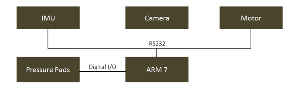
This section describes the hardware used in the biped roots. Each of the robots consists of mechanical hardware, sensors and central processing unit. Figure 1 shows the overall system. Mechanical hardware consists of robot frame and structure and the servo motors. The frame and all the mechanical structure is made from aluminium alloy sheet metal to keep the weight of the robot low while maintaining rigid structure. The motors used are Kondo KRS 4014HV. The robots consists of 22 degrees of freedom and it is connected together through RS232.
The central processing unit used is ARM-7 [60 MHz] RISC microprocessor. All the processing and intelligence will reside there. It gets the inertia data from the IMU, camera and communicate to the motor through serial at 115.2 kbps. The processing unit also processes and computes all the necessary information using the all the sensors.
The sensors suits chosen are our own inhouse developed camera system using Texas Instrument chip, 3 axes commercial off the shelf IMU (3 axes accelerometers +/- 2g, 40 Hz bandwidth, 3 axes rate gyro +/- 100 deg/s 30 Hz bandwidth, 3 axes magnetometers (+/- 750 mgauss), pressure sensing pads.
The three axes IMU have in-build Kalman filter to give correct attitude. It is capable of providing attitude information at 100 Hz. The high update rate will enable the robot to balance and also process the information.
2 Humanoid Robot Structure
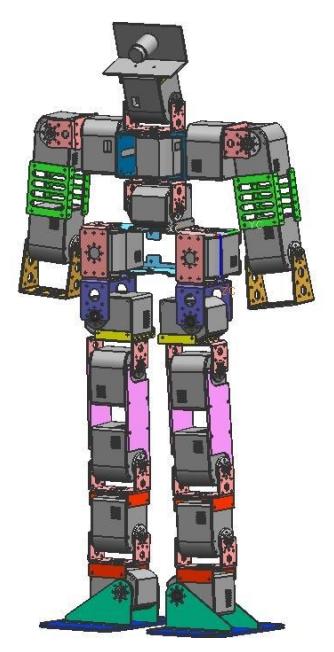
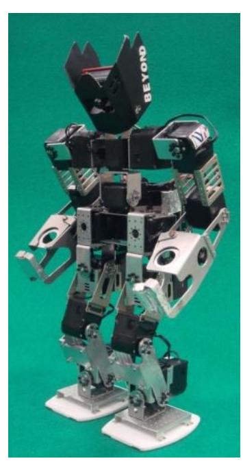
The humanoid robot in Figure 2a is used in our experiments. The robot is developed by the Mechantronics System and Integration Group, School of Engineering(Manufacturing) at Nanyang Polytechnic. Our work concentrates on the lower abdomen of robot balance.
The mass distribution of the humanoid robot is mainly in the upper body. The hip motion mainly determines the trajectory of the center of gravity (COG) or the Zero Moment Point (ZMP) of the robot. The humanoid model has a left hip joint and a right hip joint with a hip link between two hips joints. The main planning of walking gait is based on achieving motion for an unstable platform.
2.1 Unstable Walking Cycle for a Biped Robot
Many articles show how to stabilise a humanoid robot gait by modifying the motor positions in order to maintain the ZMP within the convex hull of the foot support area [1]. Table 1 figure (a) is the resting or initialisation posture. As seen in the figure, the robot is initialised with the knee slightly bent.
Table 1 figure (b), (c), (d), (e), (f), (g) and (h) show a typical walking cycle. The walking cycle starts from time T^0 at k steps. Each step takes 500 msec. The approach is to apply the instability of the robot to make the robot walk faster. However, by doing this there is a risk that the oscillation frequency of the robot is excited. This will make controlling of the robot more difficult. Various experiments were conducted on the robot by varying the values of the percentage of ZMP and the results are summaries in Table 1. From the results tabulated in Table 1, the most feasible solution range from 30 - 50 % of ZMP. This results an sideway oscillation of 1 Hz and a step size of 7.2 to 5.0 cm. Figure 3 illustrate the walking sequence and the programming logic.
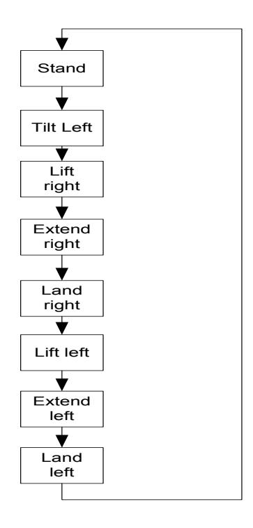
Table 1. Walking cycle
| Front view | Right side view | Front View | Right side view |
|---|---|---|---|
| Stand (a) | Tilt Left (b) | ||
| Lift Right (c) | Lift left (d) | ||
| Extend Right (e) | Extend Left (f) | ||
| Land Right (g) | Land Left (h) |
Table 2. Experimental Results of ZMP
| ZMP | 30% | 35% | 40% | 45% | 50% |
|---|---|---|---|---|---|
| Step size (cm) | 7.2 | 6.5 | 6.1 | 5.4 | 5.0 |
| Linear Speed (s/m) | 7.3 | 7.8 | 8.4 | 9.1 | 9.9 |
2.2 Universal Walking Gait
A set of universal walking gait was created. This set of gaits enables us to reduce the code size buy reusing the code. By changing a set of parameters, the same set of sequences can be used to walk straight, turn-around, side-step. This research work is still under investigation to evaluate the effectiveness and performance in speed.
3 Robotic Vision
Our research field in this area can be categorized into three different stages, namely: identification, localization and integrated control.
3.1 Identification
The identification of objects in vision primarily uses colour recognition. We have been using common colour systems like RGB and HSV to recognize objects of different colours. The problem arises when objects of similar colour, having very close coordinates in the colour system, appear in the same image. We are looking into algorithms that could recognize the shapes and other attributes, like texture, of an object, so that the recognition process does not depend solely on colours.
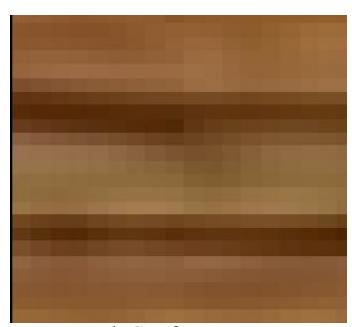
For texture recognition, we are developing a "Divide-and-Conquer" algorithm. The object image is broken up into segments of say 32 x 32 pixels. Each segment is then closely examined for its "roughness", that is, the continuity of the colour coordinates. A rough surface would have larger bands of similar coordinates, whereas smooth surface would have either entire segment with similar coordinates or smaller bands. See figure below. The information of individual segment is then pieced up, checked against previously acquired parameters to determine the type of the object.

3.2 Localization
Once the objects are identified, relative position of the object to the robots will need to be determined. Numerous methods can be used. However, with our experiments, methods that depend on the calibration based on coordinates of the centroid or the size of the object in the image have been tested and found to produce favorable results in terms of reliability on the position.
3.2.1 Static Calibration Method
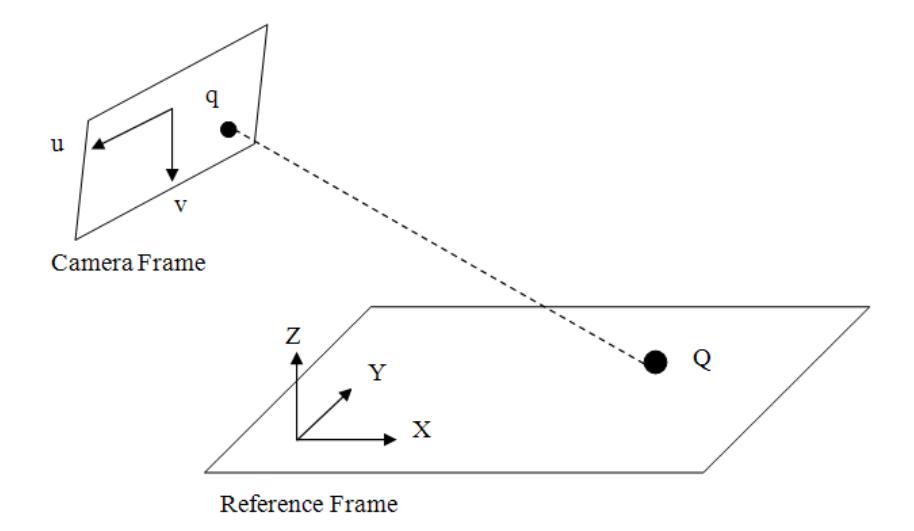
The calibration method developed involves a single transformation between the reference frame and the camera frame (Figure 5).
The equation used can be reduced to the form:
$$\begin{bmatrix} kX_r \ kY_r \ k \end{bmatrix} = \begin{bmatrix} a & b & c \ d & e & f \ g & h & 1 \end{bmatrix} \begin{bmatrix} u \ v \ 1 \end{bmatrix}$$
where the transformation matrix for a given configuration is a 3x3 constant matrix.
Using the above transformation matrix, calibration method was developed to accurately calculate 8 unknowns' values in the transformation matrix, with an error of less than 1cm in an area of about 1 m2.
3.2.2 Dynamic Calibration
The problem with static calibration is that once the orientation of the camera is adjusted or shifted, the calibration matrix obtained cannot be used anymore. AS a result, dynamic calibration methods that are independent of the orientation of the camera, was developed. This method in our option is more suited for our biped robots.
3.2.3 Estimation and predicting the velocity
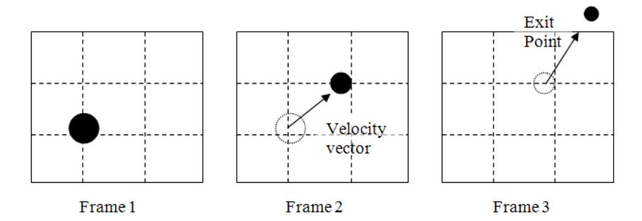
In this section, we look into the possibility of using the static calibration method mention in 3.2.1 to predict the velocity of a moving object. The assumption we made is that there is no significant change in acceleration between subsequent frames when the image is capture. Using the calibration method described in section 3.2.1, velocity (speed and direction) of the moving ball could be calculated from frame to frame. See Figure 5. By considering the size of the object image, we can also estimate the distance from the camera, and this can be used as a confirmation of the calibrated results. By dividing further the camera frame into 9 parts, together with the knowledge of the position of the object in previous frame, the exit point can be determined should the object move out of the field of view, and the algorithm can then orientate the camera to follow or track the object accordingly.
Kalman/Kalman Bucy filter has been widely used in inertial navigation. Thus will be interesting to evaluate if Kalman or Kalam Bucy filter can be used in predicting the velocity when the moving path of the object is non-linear.
3.3 Integrated Control
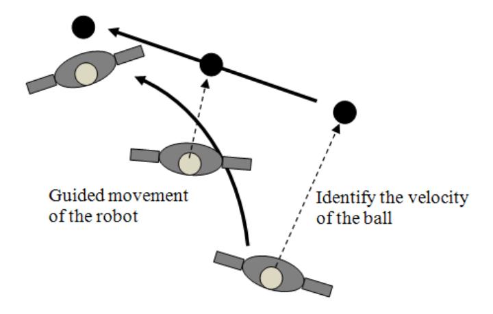
After knowing the relative positions and velocities of objects, the next step is to develop motion control systems, with vision as the feedback input, to guide the movements of the humanoid robot. One example is to line up the robot with the moving ball and the goal post dynamically, with the knowledge of the position of the goal and the velocity of the ball.
This method borrowed from a traditional guided system (proportional navigation guidance) [2] where the heading angle rate is made proportional to the LOS (line of sight rate). This algorithm is adapted where the robot's movement is homing towards the moving object. See Figure 7. With the consideration of the velocity and acceleration of the moving object and that of the robot, the robot is guided to intercept the ball (if the ball is moving with reasonable velocity and acceleration). We will have a set of different speed controls for the robot (slow, steady gaits up to fast, dynamic gaits), so as to mimic acceleration control, to be used in the guiding process.
The common challenge for all three stages is to perform the computation in real time. Since the robot moves with dynamic gaits, the communication between the camera system and the main controller cannot have a long time-lag.
References
[1] V.Prahlad, G.Dip, C.Meng-Hwee, Distrurbance Rejection by Online ZMP Compensation, In Robotica (2008), Volume 26, pages 9-17. Cambridge University Press, United Kingdom. [2] C.F.Lin, Modern Navigation, Guidance, and Control Processing, Prentice Hall.