Bahia2D 2010: Team Description
Bruno Silva, Diego Frias, Igor Eloi, Jose Grimaldo, Marco A. C. Simões
Bahia State University (ACSO/UNEB), Salvador, BA, Brazil
Abstract The Bahia2D is a Brazilian team started in 2006 that took part in two RoboCups. Currently our research aims to create computational models that allow prediction of agents' actions on the world, leading to a better decision model. This paper describes pass model creation and the necessary infrastructure to create experiments and collect information regarding its results on the environment. We also describe the initial results and future directions.
1 Introduction
The Bahia2D team is developed by the Computer Architecture and Operating Systems Group, within the line of research Intelligent Robotics that focus on research, analysis and development of solutions on intelligent robotics. It is one of three teams that compose the Bahia Robotics Team (BRT), which looks for solutions on the above outlined goals through robotic soccer researches, cooperatively lining up with RoboCup international research initiative. Currently, the group also develops teams for Simulation League 3D and Mixed Reality. Bahia2D was the first, being started in 2006, and participating of world RoboCup's in 2007, at Atlanta, and 2009, at Graz.
Since the project's beginning, our team makes use of knowledge [1] and base source code provided by UvA Trilearn. Our initial effort, that continued until last year and is summarized in our 2009 TDP, was to develop the agent's ability layer through neural networks and, mainly, fuzzy logics. Last year, the group focused on trying to develop a generic framework for soccer playing agents that could be used (when extended) by three categories in which we participate, however, after four months of project, we identified the need of more mature knowledge about the three envinronments, a consequence of such framework complexity. Such event initiated the team's present phase, focused on achieving environment's understanding and analysis; developing models that describe world's behavior so agents can use them in the decision making process; as well as in the necessary infrastructure to create rigorous experiments over soccer 2d environment. From these studies, we intend to develop a new architecture to our agent, in order to replace the already old present structure. The remainder of this paper details the first step of this process, from infrastructure building, the tests, up to the first studies on a passing model, and future works.
2 Pass analysis
To master passing ability is basal to a soccer team to show a good performance, being this ability one of the bases to execute offensive moves and maintain ball possession. Discontent about our agent's passing ability, we chose it as the focus of our study.
Essentially, a pass is the ball passage within possession of an agent, to a point in the field where a teammate can recover it with better conditions to achieve the team's present goals. Obviously, it is important to avoid that an opponent catch the ball during this move. We decided then to build a model that would foresee the chances of the ball not being captured by an opponent player, given a certain trajectory from A to B, allowing us to evaluate risks involved in a pass.
2.1 Ball Interception Model
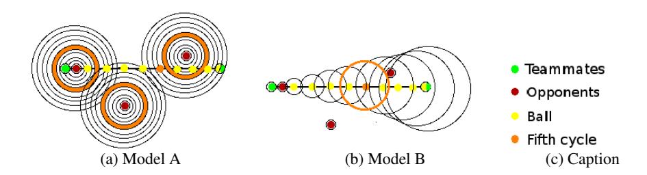
The creation of the passing model requires some issues to be completely understood, the first consideration is related to the discrete time of the environment. This creates a situation where the ball don't need to go through all the points of the trajectory to reach its destination, the ball can even "jump" a player, making it harder or even impossible for this player to capture the ball. The second point relates to identifying the players that could intercept the ball, given its initial velocity, before reaching its destination. This limitation depends on their position, orientation and initial velocity of the interceptor, additionally their physical limits i.e: maximum speed, body turn ability. To simplify the implementation our model considers the interceptor as moving at the server maximum speed in any direction (a circle around the player), in a circular distribution.
These characteristics guided the development of a model that, at every cycle, follows the possibilities of movement of the ball and interceptors (with the simplifications above). This allows identifying if is statistically possible to capture the ball when the logical circle around the player in the cycle t overlaps with the point where the ball is on the same cycle. This situation is demonstrated on the Figure 1a.
2.2 Mathematical Model
Consider a player at position $p=(x_p,y_p)$ into the field who needs to evaluate the success probability of the ball to reach a given point $f=(x_f,y_f)$ into the field arriving to that point with a final velocity $v_f$. Let $v_0>v_f$ be the initial velocity of the ball at p, to be determined, and denote by $a_k=(x_a^k,y_a^k),\ k=1,2,\ldots,n_a$ the position of the k-th adversary at the pass moment, where $n_a$ is the number of adversaries in the field.
Consider a time discretization prefixed by the server cycle duration $\Delta T\left[s\right]$ in such a way that all variables are updated at cycle times $t={0,\Delta T,2\Delta T,\ldots,m\Delta T}$ where m is the number of cycles needed to the ball reach position f, or its closest point, having a prefixed velocity $v_f$ at the arrival moment, starting from position p with a given initial velocity $v_0$. It is considered that the ball depicts a linear trajectory and starts at time t=0 and that the initial velocity of the ball is limited by $v_{max}$. We consider a continuous decrease in ball velocity according to server parameter $ball_decay$. Therefore we have that the initial velocity must satisfy $v_f \leq v_0 \leq v_{max}$.
Calculation of the Success Probability The success probability depends on the number and positioning of the adversaries close to the trajectory of the ball, that is close to the line joining points p (initial) and f (final) in the field plane. More precisely, it depends on the distance of the adversaries to the discrete positions where the ball is expected to be at each cycle time, lets denote it as $b = {b_0, b_1, \ldots, b_m}$, where $b_0 = p$ and $b_m \approx f$. Considering that the time the ball needs to reach the position $b_i$, $i = 1, 2, \ldots, m$ is $t_i = i\Delta T$, we have to consider only adversaries that at time t = 0 are at distances $s_{k,i} < i \ v_a \Delta T$ from $b_i$, where $v_a$ is the average velocity of the adversaries and $k = 1, 2, \ldots, n_a$ is the identification number of an adversary located at position $a_k$ at time t = 0. In other terms, we must consider all the players k that at cycle i satisfy $s_{k,i} = ||a_k - b_i|| < i \ v_a \Delta T$, $k \in {1, n_a}$.
Let $P(k,i) \in [0,1]$ be the probability that adversary k intercepts the ball at position $b_i$. Therefore the ball scape probability from player k at position $b_i$ is given by 1-P(k, i). This way the success probability can be formally written as
$$P_s = \prod_{i=1}^m \prod_{k=1}^{n_a} (1 - P(k, i))$$
To complete the model we must define a function that allows calculate P(k, i) as a function of the distances sk,i. Among others we choose
$$P(k,i) = \frac{s_*}{s_{k,i}}$$
for s* < sk,i < i va∆T, with the bounds, P(k, i) = 1, for sk,i ≤ s* and P(k, i) = 0 for sk,i > i va∆T.
The values of s* and va, even that naturally limited, can be adjusted for better performance of the estimator. For example, for teams with good defense the values of s* and v^a must be higher than that for a team with poor defense. In the section 4 we show the results obtained for several experiments that were carried out to evaluate our probabilistic model.
3 Planning the experiments
[This section contains subsections only]
3.1 Offline coach infrastructure
To correctly evaluate the probabilistic model an automatic and as far as possible reusable experimentation method is necessary. As creating a reusable structure is a difficult problem in software design, with this in mind we took an iterative development approach, designing a set of classes focused only on the two-dimensional simulation. This allowed a faster and more focused initial implementation and a better understanding of the requirements, which will, in the future help in creating a more general solution.
In this implementation, the experiment represents a given situation in game, for example, a corner kick with three teammates on the opponent's area. Every experiment has a single sample type and a number of samples, each sample is formed by data regarding objects involved, their positions and initial formation, there is also the analysis methods, and its result generation (output). The experiment itself, after all samples have finished, calculates statistics obtained from the their execution i.e.: average value.
The experiments are managed by the LabManager, which controls all the pending experiments and guarantees that if it is interrupted by end of match or adverse conditions the pending experiment will be restarted on the next execution.
3.2 Performed experiments
We perfomed controlled experiments, aimed to rebuild, using the structure defined in Section 3.1, pass situations that could represent the set of possible passes in a match. They were created in a controlled manner and repeteadly executed in order to obtain a statistically valid result.
This experiment objective was collect data regarding the model's precision, enabling its evaluation and refinement. This refinement was conducted through comparison of the predicted success rate and the obtained results in the simulation for the test cases. The dependent variable of this experiment is the pass success rate obtained in a given simulated situation. The independent variables are the opponent's position and the opponent team overall quality. The number of opponents was controlled, and always set to one, the distance used was eightenn meters, initial velocity 2.5 m/cycle and the direction of the pass, accepting a maximum of three degree variation on the error.
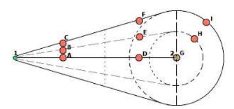
The agents positioning in an experiment are handled by an envelope surrounding the circles originated from the ball at each cycle as shown in Figure 1b. Inside this envelope the positions close, medium and far were defined for the horizontal and vertical axis. The nine positions seen in Figure 2, named from A to I are generated from this logic.
4 Experimental results
Based on the results obtained, presented on Table 1, we can infer the model was more conservative then reality, even so, the results showed a positive consistent variation of the values. From these results we can understand the importance of adding the adaptability to the model based on the current opponent's perfomance.
4.1 Evaluating the Probabilistic Model
For each experimental case we computed the success probability P^s using the model and recorded sample result, as TRUE if the ball was not intercepted and FALSE when it was. We defined two P^s classes: Theoretical True class, when P^s exceeds the value Pmin = 0.65 and Theoretical False class when P^s was lesser than Pmax = 0.35, in such a way that Pmin ≥ Pmax. We then defined a model quality criteria Q given as the ratio of good predictions with respect to wrong predictions, that is Q = Ngood/Nwrong.
Table 1: Results from experiments calculating the success average of a pass eightenn meters long with one interceptor and repeated a thousand times
| Set | Predicted success ratio | Success against opponents ratio | ||
|---|---|---|---|---|
| WrightEagle | PET-Soccer | KickOffTug | ||
| A | 0.162 | 0.270 | 0.143 | 0.530 |
| B | 0.256 | 0.396 | 0.492 | 0.517 |
| C | 0.695 | 0.623 | 0.947 | 0.765 |
| D | 0.042 | 0.009 | 0.109 | 0.242 |
| E | 0.285 | 0.301 | 0.450 | 0.817 |
| F | 0.549 | 0.816 | 0.939 | 0.992 |
| G | 0.000 | 0.328 | 0.222 | 0.091 |
| H | 0.559 | 0.834 | 0.755 | 0.588 |
| I | 0.793 | 0.987 | 0.964 | 0.989 |
In this case, Ngood counts the experiments considered as Theoretical True and had a TRUE result in the sample plus the experiments considered as Theoretical False and had a FALSE result. Nwrong counts the experiments where the predicted Theoretical class was opposite to the sample result. In an stochastic case Q = 1 because the model does not reflect the success probability at all. As Q increases above 1 the fitness of the model increases, which allows choosing optimized parameter for the model, in particular s* and va, as shown in the Section 2.2. According to results presented on Table 1 and above criteria we obtained the following value Q = 7443 + 5275/4557 + 725 = 2.41.
We consider these good results for a first approach, despite the significant deviation on the TRUE results for Theoretical False experiments. This gives further data to conclude that the s* value generates a too conservative model, needing fine-tuning.
5 Future Work
In the short term future we plan to create experiments with smaller chances of disturbing players world model. Another goal is to improve the model, so that it can be seamlessly integrated into the agents, taking into account uncertainty and heterogenous types.
There is also a long term goal wich aims to gradually improve the information collection from the agents, by means of communication with teammates and coach and using a more accurate neck control. Incrementally building a base of experiments to solidify the information gathering from matchs and situations.
References
- de Boer e J. R. Kok, R.: The incremental development of a synthetic multi-agent system: The uva trilearn 2001 robotic soccer simulation team. Master's thesis, University of Amsterdam, The Netherlands (Feb 2002)