Alice2022: Team Description Paper
Fan Wang, XueTao Lin, Yu Xiao
Robotics and Innovation Technology Lab School of Computer and Information HeFei Normal University, P. R. China
Abstract This team description paper mainly explains the work of Alice2D at this stage. According to the characteristics of our team , based on past research, our team is committed to studying the Monte-Carlo tree algorithm and reinforcement learning algorithm. Changes to defense strategy optimization. After many tests, we continuously optimize the team code, which has greatly improved the performance of the court.
1 Introduction
Alice2D was founded in 2016, by the Hefei Normal University Student Innovation Laboratory of a group of robot-loving soccer students. Our team code is based on Agent2D3.1.0 [1] which was released by Hidehisa Akiyama. It also includes fragments of released code of Marlik12[2]. On the basis of the accumulation of data left by the former Alice2D captains, after several rounds of code iteration, the unique version was finally formed. We sincerely thank all the open source developers involved for their help in lowering the bar for us to participate in 2D competitions. In the 2017 World Tournament, the team won the seventh place in the regular season and won the championship in the challenge, 7th place in the 2018 World Cup regular season. In China, our team is also named Miracle, winning the third place in China division of the 2019 RoboCup World Cup and the third place in China division of the 2021 RoboCup World Cup.
2 Related Work
Here, we will study the chapter published by the 2D team. Cyrus2D team studied using the server's full state mode to obtain the data set to predict the full state behavior of the ball holder and optimize the perspective of the agent. FRA-UNIted team studies the use of deep Q-learning (DQN) algorithm to improve the learning speed of agent. Helios2021 team is committed to considering the ability differences between their own players and their opponents to exchange players' positions, so as to optimize the role allocation of heterogeneous players. Yushan 2021 implemented the digital twin framework, used HFO tools to build the overall portrait of the team, and conducted in-depth analysis for the key areas of attack of different teams on this basis.
These theories helped us develop the idea of modifying the source code and evaluate the changes by running the game against the relevant binary pieces.
3 Block based on Monte Carlo tree search
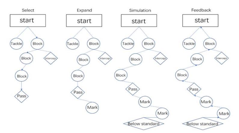
During the match, the ball handler's actions are ahead of other players, due to the mechanism that players can accurately know their own actions and situations during the T period, but the understanding of others can only come from the notification offered by Soccer Server during the T+1 period. Therefore, if our players only take actions that correspond to the opposing ball handler's actions, there may be a delay of one or more cycles. However, using Monte Carlo tree search to predict outcomes can solve this problem. Monte Carlo tree search algorithm consists of four processes: selection, expansion, simulation and feedback. During the selection process, we assume that the Monte Carlo tree will start when the opposing team takes possession of the ball and enters our player's territory, or when the opposing team gains possession of a special mode ball to stop the game. Then the child node of the Monte Carlo tree is the state transition generated by the state prediction after the defensive action output by Agent in the competition. In other words, the child node is our simulation of the defensive action. The search algorithm starts at the root node and selects a path to the leaf node (a state that meets the expected value or is below the standard value, for example: The enemy passes the ball, we trigger the interception logic, etc.) according to certain policies, expand the leaf node and do Monte Carlo simulation, record the results at the same time, and finally update the value of the node according to the path of the simulation results. The success rate for each simulated state is the ratio of the number of times the node achieves the expected payoff action to the number of times it is traversed.[4]
4 Decision of shooting based on SVM
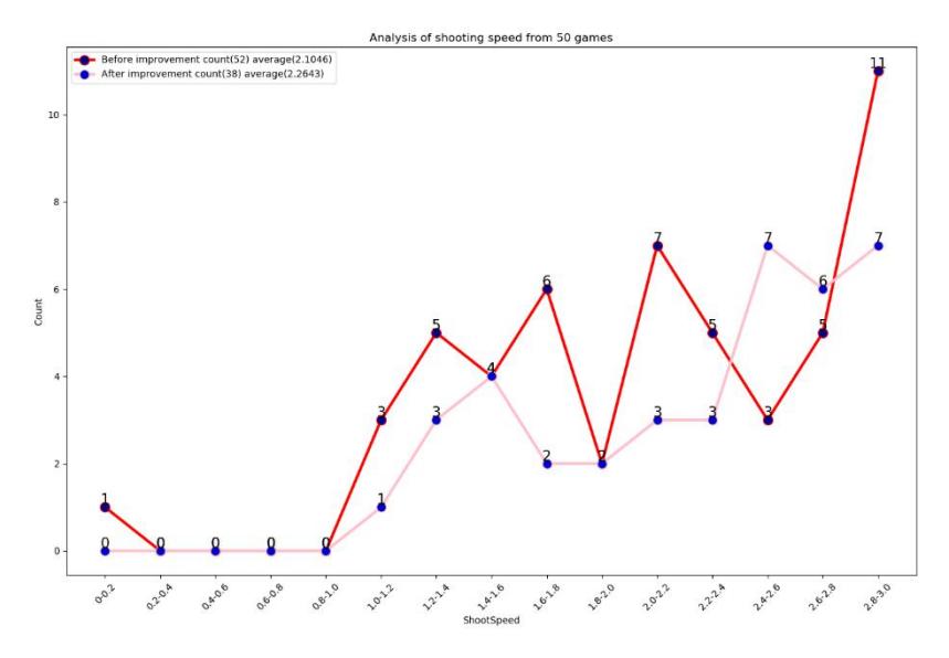
Shooting has the same nature as passing and intercepting, it is a confrontation with the opposing defender and the goalkeeper. Based on data mining techniques and 2,000 games of Alice2021 versus Helios2021 and Cyrus2021, we found that high speed shooting increased the success rate of field goals.[7]
We will consider the shooting points from the goaliepos, goalievel, goalieNeckangle, goaliebody, ballpos, ballvel, offsenseNeckangle, offsensbody, the distance between the ball and the goalkeeper, the position of the opposing player seen in the forward's visual range, and so on. And since different teams have different defensive strategies in the penalty area, it is difficult for us to predict the movements of opposing defenders and goalkeepers. According to the one-step ahead model, the analysis of the success rate of shots should be based on the state of the ball, the opposing defenders and goalkeeper in the following period. Although we cannot predict the other's actions, it is possible to predict that from the next cycle, the fastest cycle the opponent can intercept the ball. As long as the ball crosses the goal line in less time than the opponent can intercept it, the ball can break the defense. Based on this basic idea, we classify the ball that can break through the defense and the ball that cannot break through the defense, and try our best to find the hyperplane with the greatest credibility. Due to noise and random error, it is not absolutely possible to determine the initial speed of the ball after it is kicked out, and the prediction of the opponent is based on the state of the ball after it is kicked out. Therefore, N samples are evenly collected for the possible speed of the ball after being kicked out, and the interception analysis is carried out. We take that the ball can pass through the opponent's defense as the expected state, assuming that M samples meet the expected state, then the probability of successful shooting is
$$P = \frac{M}{N}$$
We first normalized N data samples, and then selected gaussian radial basis function as k ernel function for truncation analysis, namely
$$k(x_i,x) = exp^{[iii]}(-\frac{|x_i-x|^2}{2\sigma^2})_{[8]}$$
$\sigma$ depending on the speed of the shot, $x_i$ consists of Ballvel, Dist, and Angle. Based on the results of the interception analysis, we then search for the hyperplane with the greatest reliability from factors such as goaliepos, goalievel, and goaliebody. The distance calculation formula is as follows:
$$d = \frac{\omega^T x + \gamma}{\parallel \omega \parallel}$$
X is the coordinates of the support vector sample points, and $\omega$ and $\gamma$ are the parameters of the hyperplane equation.
Experimental results show that compared with the SVM method, the former improves the success rate of shooting with a threshold value.
5 Judgement on the offensive and defensive situation of the team based on reinforcement learning
In the game, the team formation has three states: offense, defense and transition. Since teams use different formations on offense and defense, players have different bases. If the player cannot identify the offensive and defensive state in a timely and accurate manner, it will cause the efficiency of the execution of the running logic of the player to be reduced due to the distance between the wrong base and the correct base, thus affecting the overall strength. [3,6]
Agent2D determines the offensive and defensive situation mainly based on the shortest interception period of players. However, teams are prone to misjudgments due to noise, heterogeneous types, and random errors during matches. Therefore, we use more diverse factors to determine offensive and defensive situations.
5.1 The Basic Process of Reinforcement Learning
In Markov decision processes (MDP), the agent can perceive the worldmodel as the current environment state, and can execute any action in the action set. In the T cycle, the environment state is $S_t$ . After the agent selects the $A_t$ action to execute, the environment state $S_t$ changes from to $S_{t+1}$ , and the $S_t$ action to execute, the environment state $S_t$ changes from to $S_{t+1}$ , and the $S_t$ action to execute, the agent at the same time. In each subsequent cycle, the agent iterates repeatedly until it reaches the final state. The action evaluation function $S_t$ represents the maximum attenuation cumulative mean value obtained after the agent selects the action $S_t$ in the state, that is, the feedback reward obtained after the agent executes the action plus the value that each cycle follows the optimal strategy. The formula is expressed as:
$$Q(S_t, A_t) = R(S_t, A_t) + \gamma \max_{t \in A_t} Q(S_{t+1}, A_t)$$
where $\gamma(0 < \gamma < 1)$ . In order to make Q-learning converge in an appropriate period, it is necessary to add an appropriate learning rate to the formula. After introducing the learning rate $\alpha$ , the formula of Q learning algorithm can be expressed as:
$$Q(S_{t'}A_t) = (1-\alpha)Q(S_{t'}A_t) + \alpha(R(S_{t'}A_t) + \gamma maxQ(S_(t+1),A_t))$$ Where $\alpha(0 < \alpha < 1)$ .
5.2 State Description
There are many factors to be considered in the process of state transition. In most cases, when the offensive state changes to the defensive state, there will be such a situation: our
offensive line is near the enemy's restricted area, the defensive line is near the midfield line, the sum of the distance between the ball and the two lines is at a large value, and the ball quickly approaches the defensive line; Most of the players from both sides gathered near the enemy's restricted area. When changing from defensive state to offensive state, you only need to replace the marker values such as offensive line and defensive line of both sides
The final state of defensive state can be described as that most of our players return to the standard point; Can perform other defensive tasks; We regain the ball right; There are special modes (ball out of bounds, foul, etc.).
The final state of offensive state can be described as our goal; The ball is intercepted by an enemy player; Special mode appears (same as the final state of the defensive state)
5.3 Action Set
The action set is a collection of advanced individual actions that can be executed by the agent. The action set can be expressed as: {Intercept, Block, Tack, Mark, Assistdefense, Formation, Shot, Pass, Cross, Dribble, Selfpass}
5.4 Determination of Reward
Take the transition from offensive state to defensive state as an example, Reward = Basic Reward + Internal Reward. The basic reward refers to the artificial division of areas. The closer an area is to the ball, the higher the basic reward. The internal rewards are mainly determined by the distance between the ball and the offensive line, the defensive line, the average distance between the players on both sides, etc.
5.5 Updated Q Value
The Q value update formula in this paper is:
$$Q(S_{t}, A_{t}) = (1 - \alpha)Q(S_{t}, A_{t}) + \alpha(R(S_{t}, A_{t}) + \gamma \max Q(S_{t}, t + 1), A_{t}))$$
When the environment reaches the final state, the Q value can be updated once according to the above formula.
5.6 Application
The fast execution of attack defense transformation can effectively prevent the occurrence of throughpass, combined with data mining and linear regression. We get the following formula
Suppose the ball goes from point A to point B in N cycles. So the ball's initial velocity, $v_{0}$ is
$$v_0 = distance/(1 + \frac{ball_{decay} * (1 - ball_{decay}^N)}{1 - ball_{decay}})$$ [10]
Distance represents the Distance from A to B and ball_decay represents the velocity decay rate of the ball. With this calculated muzzle velocity, we decide whether we can intercept it or not, and if not, we choose another defensive logical run. By modifying Alice2021's formula, we get a formula to calculate the interception success rate.
$$pass_{success}(d,\alpha,f,\varepsilon) = \left{ \frac{1}{(1+d)^{2}} * \frac{\alpha}{\Pi} + \frac{f * \alpha}{f_{max} * (1+d) * \Pi} * \left[ 1 - \frac{1}{(1+d)^{2}} * \frac{\alpha}{\Pi} \right] \right} * \frac{1}{1+\varepsilon} [5,9]$$
Where D is the vertical distance between the passer and the receiver, $\alpha$ is the range of vis ual Angle of the passer, F is the ability value of the passer, $\epsilon$ the interference of the playe r on the other side of the ball.
The experiment proves that it has a good effect on defending TP.Where D and F can be p rovided by Soccer Server, while
$$\alpha = \arccos \frac{(x_1 - x) * (x_2 - x) + (y_1 - y) * (y_2 - y)}{\sqrt{(x_1 - x)^2 + (y_1 - y)^2} * \sqrt{(x_2 - x)^2 + (y_2 - y)^2}} [9]$$
(x,y) are the coordinates of the passing player, $(x_3,y_3)$ are the coordinates of the receiving
player, $$(x_1, y_1) = (x_3, y_3 - 5), (x_2, y_2) = (x_3, y_3 + 5).$$
$$\varepsilon = (\frac{n}{n_0})/2$$
$n_0$ is the threshold for the number of our players near the passing player.
6 Summary and Outlook
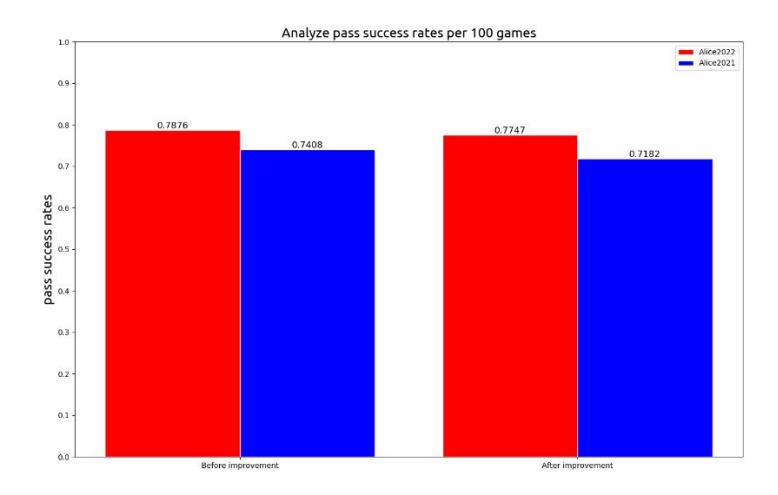
This team description paper describes the methods and algorithms implemented in the code. To demonstrate the effectiveness of these strategies, we conducted a series of computational experiments, as shown in the table below.
Table 1. Comprehensive results.
| Before and after improvement | Diff Goals | Diff Points | Game Count |
|---|---|---|---|
| Before improvement | 41 | 48 | 100 |
| After improvement | 30 | 93 | 100 |
Over the past year, our team has made improvements to formations and evaluators, continued to refine the Monte Carlo algorithm's decision tree, and made modifications to the types of players on the court in conjunction with portfolio strategy. There are still a lot of issues that need to be addressed in our team. In the future, our team will continue to improve the algorithm, optimize scripting language, data mining, log analysis and other sections, and focus on the transition from Player module to Coach module.
We will learn from other teams' strengths and improve our weaknesses. We sincerely wish the robot football simulation 2D will get better and better.
Thanks again to Mr.Cheng Zekai , Yushan team for their contribution to 2D Alliance and guidance to our team members!
References
- Akiyama, H., Nakashima, T.: Helios base: An open source package for the robocup soccer2d simulation. In:Robot Soccer World Cup. Springer. 2013, pp. 528–535.
- Tavafi, A., Nozari, N., Vatani, R., Yousefi, M.R., Rahmatinia, S., Pirdir, P.: MarliK 2012 Soc cer 2D Simulation Team Description Paper. In: RoboCup 2012 Symposium and Competitions : Team Description Papers, Mexico City, Mexico, June 2012. (2012)
- ZeKai-Cheng, NingYu-Xie, Feng-Zhang. et al. YuShan2019 Team Description Paper for RoboCup2019, The 23th annual RoboCup International Symposium, Australia, 2019.
- Zekai Cheng, Feng Zhang1 , Bolun Guang1 and Liting Wang. YuShan2021 Team Description Paper for RoboCup2021.
- Fan Wang, YuTang Guo,XingQi Zheng and XinYu Liu. Alice2021 Team Description Paper for RoboCup2021.
- CHENG Zekai,XIE Ningyu,YANG Sichun,SHE Xingxing. Application of digital twin framework based on RoboCup simulation 2D. Dec 2020.
- Yuan Song,Gan Liu,Can Wang,Zekai Cheng.Research and application of RoboCup2D log file data Mining. November 2015.
- LIU Yang,W ANG Hao,FANG Bao-fu,YAO Hong-liang.Application of the method of support vector regression in RoboCup. Oct.2007
- Potter M.A,De J.K.Cooperative co-evolution:an architecture for evolving coadapted subcomponents[J].Evolution Computation,2000,8(1):10-29.
- Yili Zhou,Xiangqin Bo. RoboCup passing strategy based on speed selection.2013.