The World Model for Autonomous 3D Soccer Agents

Hidemitsu Watanabe, Yohei Kaneda, Nobuhiro Ito

Department of Electrical and Computer Engineering, Nagoya Institute of Technology Gokiso-cho,Showa-ku,Nagoya 466-8555,JAPAN

Abstract We have participated in the RoboCup Simulation League 2D Soccer Competition. In RoboCup2005, we participate in the 3D Soccer Competition for the first time. Then, we will make use of our past experience to win the 3D Soccer Competition.

In 2D, it is very important for autonomous soccer agents to recognize correct information of other agents' positions. This is just as valid for 3D. Because they use the information to decide actions.

We construct "world model" to detect correct positions for other agents. To construct more correct world model, we focus on M. Saxena and T. Guputa's model[1]. Though there is a problem in the model, we improved the model and implemented our 2D agent on our model.

We apply our model to 3D agent and confirm that it is effective for 3D agent.

1 Introduction

We have participated in the RoboCup Simulation League 2D Soccer Competition. In RoboCup2005, we participate in the 3D Soccer Competition for the first time. Then, we will make use of our past experience to win the 3D competition. It is very important for autonomous 2D soccer agents to recognize correct information of other agents' positions. This is just as valid for 3D. Because they use the information to decide actions such as chase, dribble and so on. We construct a kind of database to detect correct positions for other agents. We call such the database "world model". And we also call it "world modeling" to construct the world model.

To construct more correct world model, we focus on M. Saxena and T. Guputa's model[1]. However, their method has a problem in world modeling. The problem causes some errors in the world model. Because it treat motion objects the same as motionless objects in their methods. So, we produced a new world modeling by dividing these two objects. Furthermore, we implemented our 2D agent on our world model. By using this world model, an error was able to be reduced even when the error is included in the information of other agents' positions. So, more correct world model was able to be constructed.

Based on the results of our model for 2D agent, we apply this model to 3D agent and confirm that it is effective for 3D agent.

2 World model

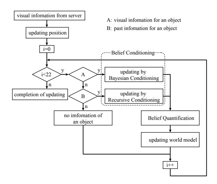
To construct more correct world model, we focus on M. Saxena and T. Guputa's model[1]. The flow of Saxena and Guputa's world modeling has become as it is shown in Fig.1. It has three features greatly as follows.

Fig. 1. The Flow of Saxena and Gupta's World Modeling

Belief Function

Belief Functions is a class of functions which is very widely used to model uncertainty, impreciseness or the provability of a state with incomplete information. We define the Belief in our case as:

$$Bel_n^{(t)}(\xi) = P(\xi_n^{(t)}|d_n^{(t)})$$ (1)

where, $\xi_n^{(t)}$ denotes the position vector of the nth player at time t and $d_n^{(t)}$ denotes the data collected upto time t, $Bel_n^{(t)}(\xi)$ denotes the Belief over the position of nth player posterior to data collected till time t.

Belief Conditioning

It is the procedure by which the Belief Functions are modified with time and with the new coming information. Belief Conditioning can be done in two ways:

- Bayesian Conditioning

It involves the estimation of the new Belief of the objects position based on the new coming data. Application of the Baye's Theorem to the definition of the Belief Function gives the following:

$$Bel_n^{(t)}(\xi) = P(\xi_n^{(t)}|d_n^{(t)})$$

$$= \frac{P(o_n^{(t)}|\xi_n^{(t)}, d_n^{(t-1)})P(\xi_n^{(t)}|d_n^{(t-1)})}{P(o_n^{(t)}|d_n^{(t-1)})}$$

$$= \frac{P(o_n^{(t)}|\xi_n^{(t)})P(\xi_n^{(t)}|d_n^{(t-1)})}{P(o_n^{(t)}|d_n^{(t-1)})}$$

$$= \alpha P(o_n^{(t)}|\xi_n^{(t)})P(\xi_n^{(t)}|d_n^{(t-1)})$$

$$= \alpha P(o_n^{(t)}|\xi_n^{(t)})P(\xi_n^{(t-1)}|d_n^{(t-1)})$$

$$= \alpha P(o_n^{(t)}|\xi_n^{(t)})Bel_n^{(t-1)}(\xi)$$ (2)

where, $o_n^{(t)}$ denotes the latest data value obtained from the server. $\alpha$ denotes the normalizing constant. The last equation suggests the Incremental update equation:

$$Bel_n(\xi) \leftarrow P(o_n^{(t)}|\xi_n^{(t)})Bel_n(\xi)$$ (3)

The conditional probability $P(o_n^{(t)}|\xi_n^{(t)})$ is called the Environment Perception Model. When the actual position is unknown we can approximate it

to be the one given by our previous Belief. Then this environment perception is the probability of new data given the estimated position. Since the new data is not as well noise free we take it's Probability Distribution Function to be Gaussian again. The prior Belief is Gaussian and the product of two Gaussian functions is also a Gaussian , this ensures the validity of the Incremental Update Equation.

– Recursive Conditioning

When no data is being received about a player during consecutive time cycles Belief cannot be modified Bayesian. We'll have to use the physics of the system to obtain the new position and velocity estimate. Moreover, the confidence over them must decrease as the time of no data increases. The Belief is centered about mean and it's spread can be estimated by variance. Therefore the following update equations are used:

Position

$$\mu_{t+1} = \mu_t + \lambda v_t \tag{4}$$

$$\sigma_{t+1} = \sigma_0(1 + \lambda t) \tag{5}$$

Velocity

$$v_{t+1} = \lambda v_t \tag{6}$$

$$\sigma_{t+1} = \sigma_0(1 + \lambda t) \tag{7}$$

Following points can be noted from these equations :

1. The confidence over the position or the velocity is given by the reciprocal of inverse i.e., the value of the Belief function at it's centre.
1. The Belief function is centered about the estimated position of the object.
1. As the time of no data(k) increases velocity decreases and therefore the object slows down.
1. Also as k increases variance increases and the function spreads out. Hence the confidence decreases.

Belief Quantification

Quantification refers to extracting out meaningful information from the Belief Function. The value of Belief Function above a threshold value is chosen for the estimation of position and velocity. If the Belief function has value less then the threshold at all positions then that Belief is discarded and a uniform distribution is assumed. This helps in saving time which would otherwise be wasted over a decayed belief Function. For our purpose we just select the best estimate which always turns out to be the mean or the centre of the Belief Function.

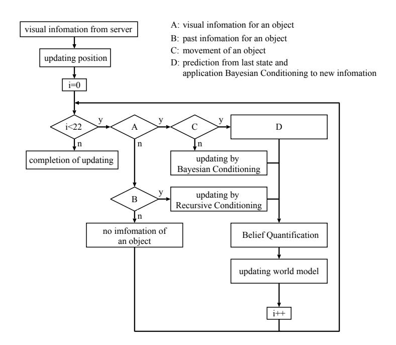
Their method has a problem in world modeling. The problem causes some errors in the world model. Because it treat motion objects the same as motionless objects in their methods. So, we produce a new world modeling by dividing these two objects. The flow of our world modeling[2] has become as it is shown in Fig.2.

3 Conclusion

We focused on M. Saxena and T. Guputa's model to construct more correct world model when we designed our 2D agent. And improving the model, we produced a new world model. Furthermore, we implemented our 2D agent on our world model. By using this world model, an error was able to be reduced even when the error is included in the information of other agents' positions. So, more correct world model was able to be constructed.

In this paper, we applied this model to 3D agent based on the results of our model for 2D agent. The same as 2D, an error was able to be reduced. So, We confirmed that our model is effective for 3D agent.

References

Manu Saxena and Tarun Gupta. Open world model for simulated soccer.2000. http://www.cse.iitk.ac.in/ amit/courses/768/00/manu/
Seiichi Furuta. Research of the world model in an autonomous robot type agent. Nagoya Institute of Technology Graduation Thesis, 2003