Little Green BATS: Team Description Paper

Martin Klomp, Sander van Dijk, Heiko Harders, A. Bram Neijt, Matthijs Platje, Mart van de Sanden, Marnix van Woudenberg

University of Groningen, Artificial Intelligence Department, Netherlands

http://alienally.mine.nu/robocup

Abstract As required for the RoboCup 3D league of 2006, this paper describes the Little Green BATS team. To implement the soccer agents, we will be using a modified version of the subsumption architecture. Simple behaviours result in a distribution of desired goal states. These are then combined by the main rule engine, which results in a single goal, which will lead to an appropriate action.

For the actual localization of the robot, the Kalman filter is used to take the errors into account.

1 Preface

We are a new team from the Netherlands called Little Green BATS. Although we are formally a private team, all seven members study artificial intelligence at the University of Groningen (RuG). It is because of our common interrest in artificial intelligence that we decided to form a team and compete in the soccer 3D simulation league. None of us had any previous experience with RoboCup, but we wanted to see how well we were able to program a team of soccerplayers with the knowledge we have gained over the past few years.

While some robocup leagues focus on creating a small team of real robots, the simulation league focusses more on higher congnitive actions. The 2D simulation league is slowly moving towards the new 3D simulation league. The 3D version is still a soccerfield with 22 players, but unlike in the 2D version, height has been added to the game. We started programming from scratch without using previous work from other teams. In the next chapters we will give a short overview of the most important features of our software.

2 Theory

(This section contains subsections)

2.1 The main rule engine

Although we deviated a little bit from Rodney Brooks specifications, most of the architecture of our robotic soccer team is based on the subsumption architecture [Brooks 1986]. Which is an incrementally extendable, behaviour based system, based on the principle of loosly coupled processes. Also we have added a few things of our own.

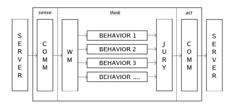
Our architecture can be devided into three parts. Namely (1) the worldmodel, (2) the behaviours and (3) the jury as can be seen in Figure 1.

The worldmodel concists of everything the agent knows about the world. The behaviours gather their input from it.

The jury is a rule based entity that regulates and combines the output from the behaviours according to gamestate specific rules, specified in a configuration file. The jury makes 'real' subsumption possible by enabling behaviours to subsume (making the jury ignore) other behaviours. This is not strictly speaking real subsumption because our behaviours are not sorted according to their 'cognitive' complexity, or any other ranking and therefore all behaviours can subsume any other behaviour.

The behaviours are an unordered set of behaviour objects. The independent behaviours cannot communicate with each other, only with the worldmodel, from which they strictly speaking only acquire input (like, the gamestate, the balls location, goalpost locations, our position in the field, etcetera). Their output is send to the jury and concists of a location, a location desire, a kick direction and a kick desire.

We decided to use location instead of a direction vector so that the jury has a little bit more information to work with. A location is either represented by a Monte Carlo distribution or a normal distribution.

Desires are values ranging from −1.0 to 1.0 for which a value of zero means that the behaviour does not want the jury to do anything with it, a value below zero means the behaviour wants the jury to do the opposite and a value of 1.0 means that the behaviour is very sure of itself and badly wants the jury to listen to it. All values in between are possible of course.

Inside the jury, samples from all location distributions are taken and put into one (big) Monte Carlo distribution. From this distribution a sample is taken. The location vector of this sample is then subtracted by the location vector which represents the agent's current belief of its position in the field. The outcome is sent to the server as the direction in which to move.

If the kick desire of a behaviour is larger then 0, all other activities are suspended and only a kick instruction is send to the server.

2.2 Localization

For many situated agents, including football playing agents, it is important to know what position they have in the world. This knowledge is needed to asses the situation and to decide what actions need to be taken to reach a desired state of the world. For the current 3D soccer simulation this certainly holds. Moreover, the dynamics of the simulation require a certain level of accuracy. Agents are only able to kick the ball if it is within a range of 4cm and the location of the agent with respect to the ball fully determines the direction the ball will be kicked to. So correct localization is one of our main concerns.

The agent receives some information that can be used for localization through its vision perceptor, namely the polar positions of the corner flags and goal posts relative to the agent. Since the agent knows the absolute positions of these objects he can calculate his own position in the field using these measurements. However, some noise is added to these perceptions, so an agent can not rely on one single measurement. The simplest way to decrease the error is by taking a weighted average over these N measurements:

$$m(t) = \frac{1}{N} \sum_{i=0}^{N} w_i \cdot x_i(t)$$

where $w^i$ depends on the standard deviations of the seperate measurements. In the simplified case of equal variances for each measurement, the variance of the averaged measurement is:

$$\begin{split} \frac{1}{\sigma_m^2} &= \sum_{i=0}^N \frac{1}{\sigma_i^2} \ &= \frac{N}{\sigma^2} \ \sigma_m^2 &= \frac{1}{N} \sigma^2 \end{split}$$

So in our case, where we have 8 seperate measurements, the error decreases by a factor of 64.

Further precision can be obtained by taking into account the movement actions of the agent performed in the world. The localization algorithms that do this can all be devided into two steps:

1. Predict the position of the agent given the previous estimated locations and the actions that were performed.
2. Update this prediction given the perceived measurements.

Often probability distributions are used to represent locations and the main difference between localization algorithms is the way they represent these distributions. Some examples of these representations are normal distributions defined by means and covariance matrici, grid based representations and Monte Carlo distributions. The latter two are popular in robotics because they are robust and can handle situations like the 'kidnap problem'. However, because these representations require quite some resources we have chosen to use normal distributions that are updated with a Kalman filter, as described by Negenborn [?].

At each cycle the filter predicts the current a priori location $N (m^{-}(t), \Sigma^{-}(t))$ given the last a posteriori location $N (m^{+}(t - 1), \Sigma^{+}(t - 1))$ and action model A:

$$N(m^{-}(t), \Sigma^{-}(t)) = N(m^{+}(t-1) + m_{A}(t), \Sigma^{+}(t-1) + \Sigma_{A}(t))$$

Next, the a posteriori location is determined by updating the a priori location with the measurement model M:

$$N(m^{+}(t), \Sigma^{+}(t)) = N(m^{-}(t) + K(m_{M}(t) - m^{-}(t)), \Sigma^{-}(t) - K\Sigma_{M}(t))$$

With:

$$K = \Sigma^{-}(t) \left( \Sigma^{-}(t) + \Sigma_{M}(t) \right)^{-1}$$

2.3 Monte Carlo

In our architecture, as described above, the jury gets its probability distibutions from the different behaviours. Our behaviours have the ability to generate normal distributions as well as Monte Carlo distributions [Neal 1997]. A Monte Carlo distribution is a stochastic, nondeterministic distribution of the places our agent wants to be. By using Monte Carlo distributions we are able to make a distribution on the field whithout being limited to the limitations of a normal distribution.

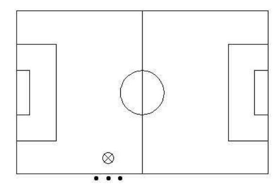
Our Monte Carlo distribution is a distribution of a number of particles in, or just around, the field. Each particle has a value between 0 and 1, representing the probability. The total of all particles should be 1 (as each probability distributions should be). Each behaviour can make as many particles as needed, as long as the sum equals 1. An example of the stayInField behaviour can be seen in Figure 2.

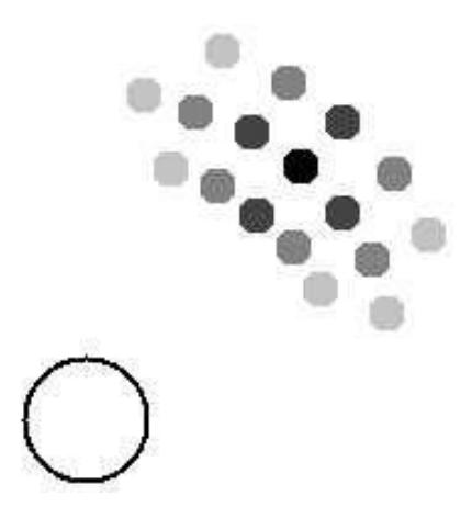
The error in the visual perceptor is polar with respect to the agent. Also, at some points, you want a probability distribution around an object (agent or ball). This can not be represented in a normal distribution. By using a Monte Carlo distribution in stead of a normal distribution we are able to make a probability distribution of such type (see Figure 3). Therefor it is possible to calculate new probabilities which include these probabilities.

3 Behaviours

Using the architecture described above, the best combination is created using the following basic behaviours.

3.1 ballTowardsGoal: Getting the ball in the goal

The ballTowardsGoal behaviour will try to get the player behind the ball and then kick the ball towards the goal. Only kicking when the ball is closer to the opponents endline then the player's.

3.2 stayInField: Keeping the player in the field

The stayInField behavior will make sure that no player leaves the field except when he will be the one kicking in the ball.

3.3 stayInFormation: Keeping the player in formation

Using an XML configuration file, each player is given a default position on the field. This default position is part of the in play formation of the team. The stayInFormation behaviour will try to get the player into this default position and keep him there. Currently this formation position is an absolute point on the field, which is also used as the starting position for every player.

During the game, the formations can change to best suite the situation. For example, when the team is ahead in the scores a more attacking formation may be chosen.

3.4 awayFromTeammates: Not getting to close to a teammate

The awayFromTeammate behavior will make sure that the players will not stick together. There will be an good distribution on the field.

3.5 awayFromOppontents: Not getting to close to an opponent

The awayFromOpponent behavior is the same as the awayFromTeammates behavior, only staying away from the opponents in stead of your teammates.

3.6 Pass: Pass the ball to a teammate

The Pass behavior will pass the ball to a teammate on the opposite side of the field.

3.7 Dribble: Dribble with the ball

The Dribble behavior wants to get behind the ball to kick towards the opponents goal. The power of the kick is limited so the player will end up behind the ball again. Dribble is only activated when there are no opponents nearby.

4 Future work

We will be implementing more behaviors for our players so they will behave better and are capabel of more complex actions. We will improve our Pass behavior and will include some defence behavoirs. In the new server, required for the world championship, the agents are able to communicate. We will use this to be better in passing the ball to the best player. If time lets us we will implement a genetic alorithm so each player can learn the best values for their actions.

References

[Brooks 1986] Brooks, R.A., A robust layered control system for a mobile robot. IEEE Journal of Robotics and Automation, RA-2 (April), 14-23; also published as MIT AI Memo 864. [Negenborn 2003] Negenborn, R., Robot Localization and Kalman Filters. On finding your position in a noisy world, A thesis submitted to the Institute of Information and Computing Sciences in partial fulfillment of the requirements for the degree of Master of Science, specialized in Intelligent Systems. [Neal 1997] Neal, R. M., Monte Carlo implementation of Gaussian process models for Bayesian regression and classification, Technical Report CRG-TR-97-2, Dept. of Computer Science, University of Toronto.