Parsian (Amirkabir Univ. of Technology Robocup 3D Simulation Team) Team Description for Robocup 2008

Mohammad Mehdi Korjani, Arman Sarrafi, Golnaz Ghiasi

Electrical Engineering Department, Amirkabir University of Technology (Tehran Polytechnic), 424 Hafez Ave., Tehran, Iran

Abstract This team description paper depicts Parsian Robotic 3D Simulation Robocup team activities performed for preparing for Robocup 2008 3D League. This paper presents a physical simulation of a 20 degree of freedom real biped robot model used in RoboCup 3D Soccer Simulation League and demonstrates its application to exploring biped motion control techniques.

1 Introduction

As we know, one of the main goals of Robocup competitions is to develop a footballer robot team, to beat humans' champion team in 2050. To achieve this overreaching goal, robotics science should improve in different aspects. Therefore, Robocup competitions are celebrated in several leagues, each of which focuses on some of these aspects. The humanoid league focuses on balancing biped robots and joint control to create human-like movements and actions. In this league, because of high expenses of creation of such robots a few team works on it. So improvements in this field will take place very slowly. Thereby we need a simulation environment and simulated robots to decrease the expenses of our experiments. The 3D simulation league was brought to world with this goal and is a suitable environment to test our ideas on the control of humanoid robots.

Because balancing of robots and making human like actions is the main challenge in this league, Parsian team has focused on these aspects and the following is our ideas about them.

In Section 2 artificial intelligence subsystem of our robots is described including the decision maker and the behavior based layer, localization is discussed in Section 3, structure of the team is presented in section 4, followed by a description of our development tools in section 5. This team description paper is finalized in section 6 with a conclusion.

2 Artificial intelligence subsystem

Artificial intelligence subsystem is divided into two parts. In the "Behavior based Layer" each robot conducts behaviors such as walking, kicking, standing up and stopping the ball. A robot takes current game state and target game state (robots and ball position, velocities, and robot orientation) as input from Decision making layer and generates the tasks to switch from the current state to the target state. It gets robots and ball position, velocities, and robot orientation as current state and generates the target state. Then it submits the current and beginner state of robots to switch to target state with the Behavior based Layer.

2.1 Decision Making Layer

Decision making layer allows the robot to move on the field and set special action such as stand up and kick behavior. The output of this layer is one of the behaviors that must be shown? in the behavior based layer.

In this section, the game is divided to three states (defensive, offensive, and general).Each state has different positioning, so robots must cooperate to decide which of them is nearest to the ball and where is the target poison of them.

2.2 Behavior based Layer

This layer takes current and target state of the robots. Destination of this layer is reaching to the target. The current state of a robot consists of the robot X and Ycoordinates, orientation, and velocity. A desired target state consists of the final X and Ycoordinates, final orientation, final velocity or power of kicking. This section contain walk, kick and stand up behavior.

The main time-consuming part of our work was the walk behavior that makes a stable, fast and omnidirectional movement. In the sequel, the main three behaviors i.e. walking, kicking and standing up have been described.

2.2.1 Walking

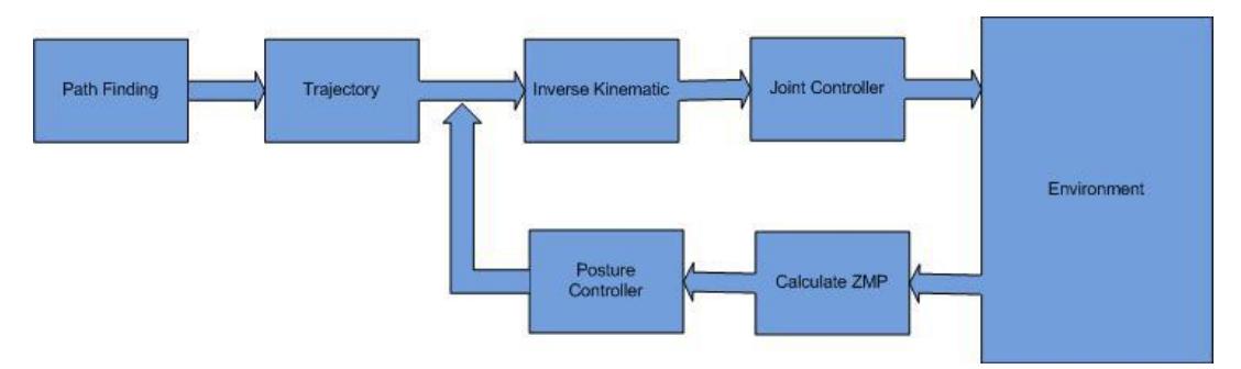
As shown in figure 1, the walk behavior contains 4 parts including path finding, Trajectory, Inverse kinematic and joint controller. In first part path finding algorithm used for obstacle avoidance and find a path to target point. After calculating next step point, trajectory subsystem find hip and foot motion curve. According to this curve inverse kinematics equation are used to calculate a posture of the robot and angle of each joint. At the end a fuzzy controller is used for smooth joint movement. By this approach stabilize walking should occur but because of environmental disturbance robots may lose their stability. Because of this we first calculate ZMP, if ZMP does not exist in 'Desired area, robot has to move a ZMP to the 'Desired area'. We do this by using posture controller and changing current angle that is calculated in inverse kinematic part.

2.2.1.1 Path Finding

To move a robot to another position, we used Path Finding which takes the current positions of the robots and the target position of each robot. This section would produce each robot's path using 'Hopfield Neural Network' [7]. Because of operation in a dynamic environment, we must use a method to overcome collision of robot. First we optimize the path by using this algorithm from the end to start and then after predicting the path from start to end. The results are very satisfactory and also the generated path is the most optimized. For avoiding the local minima, we execute the next movement energy prediction. The amount of such a prediction is variable. Hence, the amount of energy is calculated for 5 next squares for each movement. If we reach any object, the energy function will increase and optimization avoids selecting that way.

2.2.1.2 Trajectory

In this section, finding hip and foot trajectories by using genetic algorithm is described. In this approach, the key parameters which define the trajectories are searched by genetic algorithm to find the best trajectory that has asymptotical stability.

Walking is a periodic action, thus determining motion for one cycle is enough. We assume T is the period length of one walking cycle and in every cycle the foot reaches its highest position after ݐ units of time.

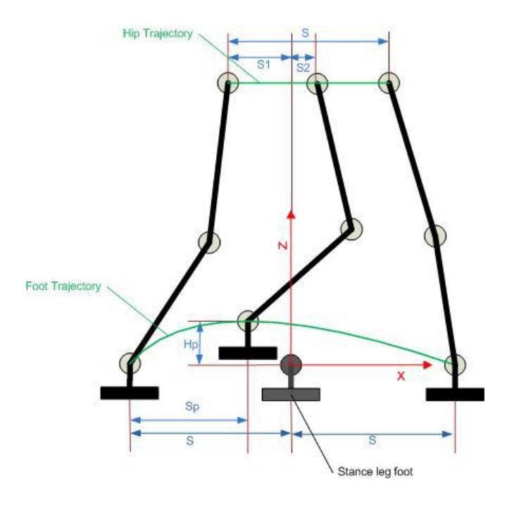
The foot trajectory parameters are shown in figure 2. As shown in this figure, horizontal position of the foot in the beginning of walking cycle is –S, in the end of cycle is S and when the foot is in its maximum heights position, ܪ, its horizontal position becomes െܵ ܵ. Besides, since the feet fully contact with the ground, the horizontal velocity at that points must be zero.

We determine 3 points of motion by using the values of ܵ, ܵ. Using these points and cubic spline interpolation, horizontal trajectory of foot is determined.

Similarly by using cubic spline interpolation and determining ܪ vertical trajectory of foot is determined.

Because the vertical motion of the hip is limited, we can assume that hip height is constant and for horizontal movement of the hip as shown in figure 2, horizontal position of the hip in the beginning of walking cycle is െܵଵ, in the end of cycle is ܵെܵଵ and when the foot is in its maximum heights position, the horizontal position of the hip becomes ܵଶ. More ever, horizontal velocity and acceleration of the hip in the beginning and ending of walking cycle should be the same. Again by using cubic spline interpolation and determining ܵଵ, ܵଶ and S horizontal trajectory of the hip is determined.

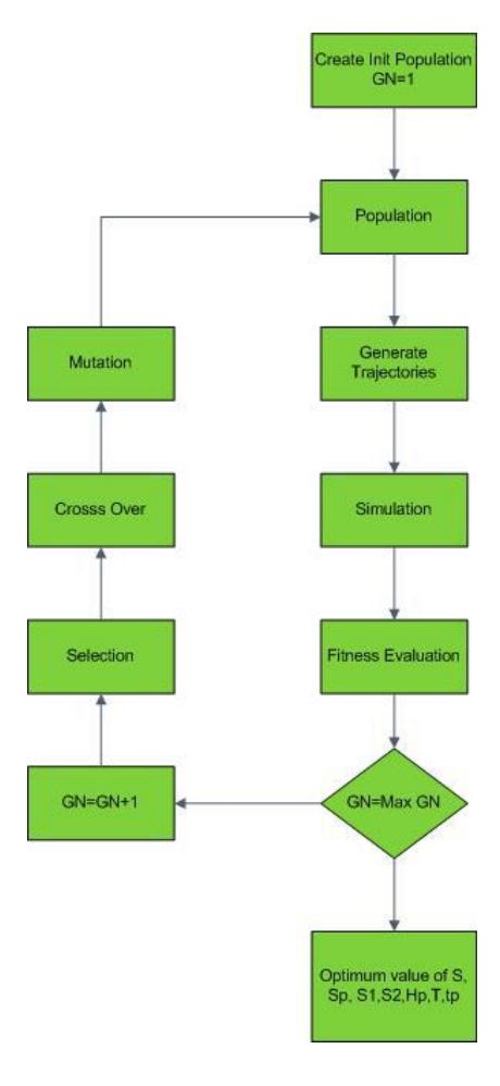
Now with genetic algorithm best values for parameters ܵ, ܵଵ, ܵଶ, ܵ, ܪ, ܶ, ݐ are determined. Fitness of individuals can be determined with regard to stability of the robot, such that the more the zero moment point is close to midpoint of stance foot in each step, the more fitness will be given. Flowchart of this genetic algorithm is shown in figure 3.

2.2.1.3 Inverse Kinematics

In walking pattern generation of the biped robot, forward and inverse kinematics equation are used to calculate a posture of the robot and angle of each joint. Kinematics analysis is based on Denavit-Hartenberg's kinematics notation. The output angle of kinematics compensate with ZMP (Zero Moment Point) compensator. Posture of a biped robot is stable when ZMP exists in 'Desired area' which is assumed as the most stable area according to ZMP. If ZMP does not exist in 'Desired area, robot has to move a ZMP to the 'Desired area'[3].

2.2.1.4 Joint Controller

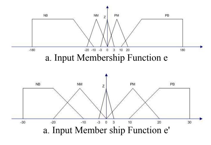
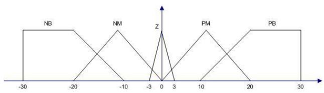
Fuzzy controller is employed to control the joint angles. Three membership functions are constructed for e and e', where e is the error between measured angle and desired angle and e' is the error between measured angle variation and desired angle variation. Each of the input variables has following fuzzy sets: NB, NM, Z, PM, PB. Membership functions consist of overlapped isosceles triangles as shown in Figure 4 and 5.

2.2.2 Kick

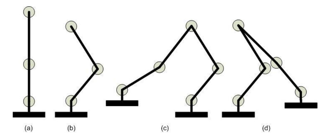
Because of keeping balance of the robot, an effective and powerful kick is a challenging task. There are two factors that influence the balance of a soccer robot in kicking. One is the quick move of the kicking leg and the other is that the center of gravity of the robot moves to the front.

Kicking action composed from three steps and figure 1 shows these steps. In the first step, the robot leans to move its center of gravity to the supporting leg and bend its legs. The robot needs to bend as low as possible to get a wider kicking range. In the second step, the robot lifts its kicking leg so high as the center of gravity remains in the supporting area. We name this height H. Finally, robot starts kicking in the third step.

For keeping the balance of the robot ankle joint angle of stance leg should be adjusted. When the kicking leg swings backward, the stance leg leans forward and when kicking forward, the stance leg leans backward. These leaning angles have an important effect on keeping the balance of the robot. We name these angles ߠ௪ௗ and ߠ௪ௗ. From these two angles. the trajectory of stance leg ankle angle can be determined by using third order spline interpolation.

Because it is difficult to go exactly behind the ball, every kick should have a kicking range that the ball can be kicked if it is in the kicking range. By determining kicking range and H, the trajectory of kicking foot can be determined similarly by the third order spline interpolation.

Thus to have an effective and powerful kicking, we should determine the suitable value for ߠ௪ௗ, ߠ௪ௗ, H, kicking range and the value of bending in the first step. These values can be determined by genetic algorithm in a similar way that we described for trajectory of walking skill. Fitness given to individuals is related to the balance of the robot and the magnitude of ball movement. After determining suitable trajectories for kicking we use similar approach as walking that described in section 2-2-1.

2.2.3 Standing up

Since in soccer games, physical contact between the robots is unavoidable, the walking patterns can be disturbed and the robots might fall. Thus the agents should be able to recognize their posture on the ground, and getting up again. From the vision data, each agent can determine its posture on the ground and regarding to its situation, it can use specific patterns for getting up. We use static patterns for getting up.

3 Localization

Every agent has polar coordinates of other objects in its vision coordinate system. However, it is better if it has the coordinates of all objects including itself in world's global coordinate system. By defining $\Sigma_A$ as vision coordinate system of the agent and $\Sigma_W$ as the world's global coordinate system, we want to find $M_{\mathrm{a}\to\mathrm{w}}$ matrix that converts the representation of a point in $\Sigma_A$ into its representation in $\Sigma_W$ . Using $M_{\mathrm{a}\to\mathrm{w}}$ , we can find representation of a point in $\Sigma_W$ by producing $M_{\mathrm{a}\to\mathrm{w}}$ and its representation in $\Sigma_A$ . In the continuation of this section, the calculation of matrix $M_{\mathrm{w}\to\mathrm{a}}$ has been described. Obviously, $M_{\mathrm{a}\to\mathrm{w}}=M_{\mathrm{w}\to\mathrm{a}}^{-1}$ .

The process of converting $\Sigma_W$ into $\Sigma_A$ is composed of two parts. First part is a transition that transfers the origin of $\Sigma_W$ coordinate system to the origin of $\Sigma_A$ coordinate system. We show this transition by T and the transition of $\Sigma_W$ coordinate system by $\Sigma_W'$ . Second part is a rotation that turns $\Sigma_W'$ to $\Sigma_A$ . We show this rotation with R.

For finding T we need to find the coordinate of the origin of $\Sigma_A$ coordinate system in $\Sigma_W$ coordinate system. We show this origin of $O_A$ to find $O_A$ we use 3 flags that we name them by $f_1, f_2$ and $f_3$ . Flags are the objects whose coordinates in both systems are known by the agent. We assume that coordinates of these flags in $\Sigma_A$ coordinate system are $F_{1A}$ , $F_{2A}$ and $F_{3A}$ and their coordinates in $\Sigma_W$ coordinate system are $F_{1W}$ , $F_{2W}$ and $F_{3W}$ . Then we have the following equation.

$$\begin{cases} |F_{1A}| = |F_{1W} - O_A| \ |F_{2A}| = |F_{2W} - O_A| \ |F_{3A}| = |F_{3W} - O_A| \end{cases}$$

In the above equation, we have three equation and three unknown variables as $O_{A_x}$ , $O_{A_y}$ and $O_{A_z}$ . Hence, we can easily calculate $O_A$ . If the unit vectors of $\Sigma_A$ coordinate system in $\Sigma_W$ coordinate system are denoted by $X_A$ , $Y_A$ and $Z_A$ , we will show that

$$R = \begin{bmatrix} X_A^T \ Y_A^T \ Z_A^T \end{bmatrix}$$

Since the rows of a rotation matrix are perpendicular to each other and magnitude of each row is equal to one, production of two different rows is zero and production of a row with itself is one. Thus, if $R_1$ represents first row of $R$, $R \times R_1^T$ is equal to $\begin{bmatrix} 1 \ 0 \ 0 \end{bmatrix}$ . Also it is obvious that $R \times X_A$ is equal to $\begin{bmatrix} 1 \ 0 \ 0 \end{bmatrix}$ . Then $R_1$ is equal to $X_A$ . Similarly it can be shown that $R_2$ is equal to $Y_A$ and $R_3$ is equal to $Z_A$ .

Thus for finding R we first find $X_A$ , $Y_A$ and $Z_A$ using $f_1$ , $f_2$ and $f_3$ . We show normalized vector of these flags in $\Sigma_A$ coordinate system with $f_{1A}$ , $f_{2A}$ and $f_{3A}$ and their normalized vector in $\Sigma_W'$ coordinate system with $f_{1W}$ , $f_{2W}$ and $f_{3W}$ . Since the length of $X_A$ and $f_{1W}$ are equal to one, dot product of $X_A$ and $f_{1W}$ is simply the cosine of the angle between these two vectors. But as $X_A$ is a vector on the x axis of $\Sigma_A$ coordinate system, the cosine of the angle between these two vectors is x component of $f_{1A}$ , means $f_{1A_X}$ . As a result, we have the following equations.

$$\begin{cases} f_{1W}. X_A = f_{1A_X} \ f_{2W}. X_A = f_{2A_X} \ f_{3W}. X_A = f_{3A_X} \end{cases}$$

And from the above equations we have,

$$[f_{1W} f_{2W} f_{3W}] \times X_A = \begin{bmatrix} f_{1A_X} \ f_{2A_X} \ f_{3A_X} \end{bmatrix}$$

Finally $X_A$ can be calculated from the equation below,

$$X_A = [f_{1W} f_{2W} f_{3W}]^{-1} \begin{bmatrix} f_{1A_X} \ f_{2A_X} \ f_{3A_X} \end{bmatrix}$$

Similarly,

$$Y_{A} = [f_{1W} f_{2W} f_{3W}]^{-1} \begin{bmatrix} f_{1A_{y}} \ f_{2A_{y}} \ f_{3A_{y}} \end{bmatrix}$$ $$Z_{A} = [f_{1W} f_{2W} f_{3W}]^{-1} \begin{bmatrix} f_{1A_{z}} \ f_{2A_{z}} \ f_{3A_{z}} \end{bmatrix}$$

All in all, the calculation of R and T has been described and using them, $M_{W\to a}$ and $M_{a\to W}$ can be calculated easily.

4 Team Structure

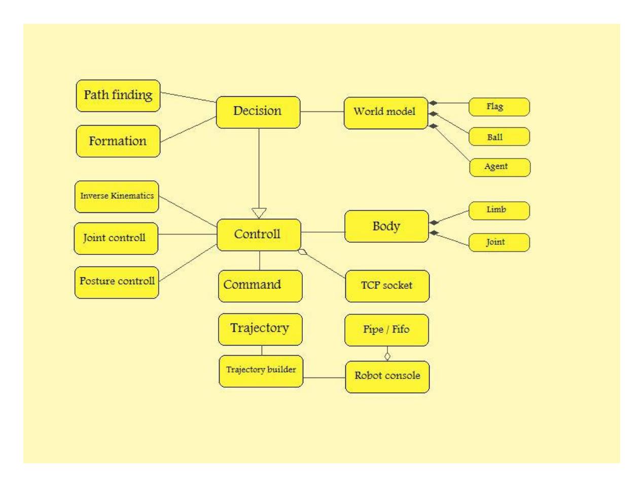
This is UML diagram of our team. It shows the main parts and their functions.

4.1 Decision class

It is the highest level layer of our team that will make decisions to go to a place or shoot the ball or stand up, then selects which trajectory must be executed. The modules of positioning and path finding are separated from decision because of their independencies to other parts. Trajectory builder is a module that builds these trajectories and will be discussed later.

4.2 Control class

When the decision algorithm selects a trajectory to run, it will be passed to the control section and it will proceed to execute it. The subsystems of inverse kinematics, joint control and posture controller are separated from this section and will be described later.

4.3 World Model and Body classes

As shown in the diagram, analyzing server messages, localization and computing of global position of external objects are done in WM. Furthermore, computation of robot limbs global positions and their velocities and computing ZMP of robot will be done in Body class.

4.4 Robot Console class

It is responsible for transferring data between agent and our assisting tools which are described in development tools section.

5 Development Tools

A time-saving and high performance tool, named trainer and monitor, is used to test server environment, train the agents and calculate the statistics of matches.

5.1 Trainer

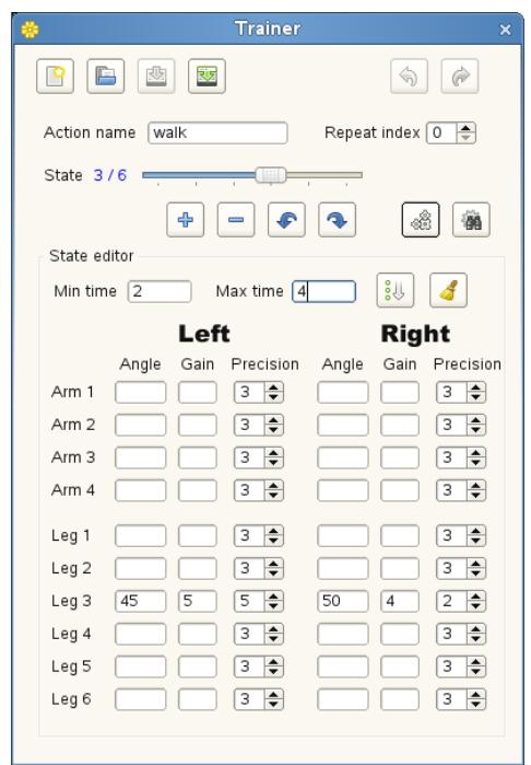
Last year, we developed this tool in team 'Aria 2007' to make trajectories manually. Its main drawback was being very time consuming. This year we improved it to match our new system and to make trajectories automatically. It will provide an environment to test trajectories created in the trajectory builder and rewards them.

5.2 Monitor

We also developed this tool last year in 'Aria 2007' team to simplify debugging our agent. This year it has been improved to show accuracy of localization, decision delay and exceptions.

6 Conclusion

In this paper, some aspects of our current team were described. Our implementation of the decision maker and behavior based layer are addressed. Three main behavior of our robot that includes waking, kicking and standing up have been described in Behavior based layer. A learning algorithm is used for optimized walking parameters and reaching fast walking steps. More ever powerful and stable kicking process is considered in this paper. In addition, the development tools that make easier our development are described.

References

1. Zhe Tang, Changjiu Zhou and Zenqi Sun, "Balance of penalty kicking for a biped robot "IEEE Conference on Robotics, Automation and Mechatronics, 2004
2. V.H. DAU, C.M. CHEW and A.N. POO," Optimal Trajectory Generation for Bipedal Robots"
3. K.C. Choil,H.J. Lee and M.C. Lee2, "Fuzzy Posture Control for Biped Walking Robot Based on Force Sensor for ZMP" SICE-ICASE International Joint Conference 2006, Busan, Korea
4. M.M. Korjani, Design, implementations and Control of a Mobile Robot in Fuzzy Environment Using Neural Networks, BSc final thesis, Electrical Engineering Department, Amirkabir university of technology, 2006.
5. T. Hemker, H. Sakamoto, M. Stelzer, and O. von Stryk. Hardware-in-the-loop optimization of the walking speed of a humanoid robot. In CLAWAR 2006: 9th International Conference on Climbing and Walking Robots, pages 614–623, Brussels, Belgium, September 11-14 2006.
6. Paul, Richard P., C. N. Stevenson, "Kinematics of Robot Wrists, "The International Journal of Robotics Research, Vol.2, No.1, Spring 1983
7. H.Y. Sun and G.Y. Tang, "Optimal Disturbance Rejection with Zero Steady-state Error for Linear Discrete-time Systems", Proceedings of the 6th World Congress on Intelligent Control and Automation, June 21 - 23, 2006, Dalian, China