Bahia3D - A Team of 3D Simulation for Robocup?
Adailton de J. Cerqueira Jr., Adriano Veiga, Diego Frias, Marco A. C. Simões
Bahia State University (ACSO/UNEB), Salvador, BA, Brazil
http://www.microsoft.com/Robotics/
Abstract One of the major challenges in the development of a soccer playing team for RoboCup Simulation League 3D, for beginner groups, is to implement movements. In this paper we introduce Bahia3D new architecture and also focus on our movement generation model. Additionally, we describe work under development.
1 Introduction
Bahia3D is developed by the Bahia Robotics Team (BRT) group, part of the Computer Architecture and Operating Systems group, that focus on investigating application of artificial intelligence methods on autonomous robots. BRT has been participating of other RoboCup leagues (Simulation 2D, Mixed Reality) since 2007, showing good results specially within Mixed Reality, in which it won third place at RoboCup 2009. This is the second year of work with 3D. In RoboCup 2009, the team has achieved 16th place in the league's overall ranking.
In the last year, our first, we have decided to develop over a base team, improving its basic skills. We therefore used Little Green Bats [1]. We adopted such approach since BRT had no prior experience with 3D basic challenges on movements. In this same year, however, because of the change on the vision system, we choose begin team's development from the very basis, since Little Green Bats base did not cover the new vision model.
In section 2 we explain our agents' new architecture. Section 3 shows two main approaches we applied to creating robots' movements: (i) Microsoft Robotics Studio [2] environment based, explained in section 3.1, and (ii) feedback approach, described in section 3.2. Section 4 describes the mathematical model designed to create movements. After that, we point out, in section 5 major obstacles encountered during our agent's development. Finally, we present achieved results and future works in section 6.
2 Architecture
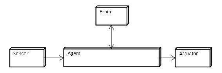
The choice of not using the Little Green Bats base code, beyond the fact that it doesn't cover the new vision model was due to a lack of comprehension on the base team's architecture. Therefore, a new architecture was designed. Such new architecture provides lower module coupling. Figure 1 illustrates our new architecture. Our agent is divided in four modules: Sensor, Actuator, Agent and Brain. Each module has specific functionalities within agent's operation.
The Sensor is responsible for capturing message sent by server and for converting it into data that the agent understands. Upon receiving a message, Sensor extracts useful information and stores it in the agent's data base.
The Actuator's role is to build and send messages to the server. The Agent informs the chosen command as well as its corresponding value, and the Actuator, on the end of the cycle, assembles the message to be sent to the server.
The Agent module works like an intermediary control module, receiving abstract actions from Brain and converting them into a particular command. For instance, the Brain sends action "kick "and the Agent translates it to a specific command, informing which joints are involved in such action and corresponding velocity so it can be achieved.
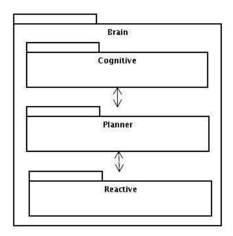
It is in the Brain where all the agent's reasoning is located. Internally, this module is divided into three interrelated layers, as can be seen in figure 2.
The Reactive level is the most basic within the Brain, dealing with execution of simpler and less reasoning actions, and executing actions arising from higher levels decisions. The Planner is responsible for analyze information received from server and for decision making based on such analysis. Subsequently, we have the Cognitive level, that plans and manages goals the team must follow, based on information acquired during the match.
We must remark that the last two layers (Planner and Cognitive) are still to be developed, and that with their implementation we expect provide a structure so the team can work as a collective intelligence.
3 Movement
One of the major challenges while elaborating a 3D simulated agent is making complex movements from the conjoined moves of each joint. To overcome this challenge, we've built a movements planning model based on MicroSoft Robotics Studio approach. The movements are controlled by a feedback model, which aims to keep robots move within planned boundaries.
3.1 Microsoft Robotics Studio based approach
The MicroSoft Robotics Studio (MSRS) simulation environment also has a simulated model of NAO robot. The simulator has some pre-defined moves and a base source code, to aid quick development of new teams.
Some months before beginning to work with RoboCup simulation 3D, the team had tried the MSRS environment and acquired some experience with it. Thus, in order to solve the robots' basic movements making within Simspark, we've decided to adopt an approach based on MSRS pre-defined movements.
A movement in MSRS consists of a sequence of static postures, separated by a certain time interval between them. Each pose determines each joint's angle related to its own axis. Nevertheless, NAO's simulations on MSRS and Simspark differ by some attributes, e.g., minima and maxima angles, joint's axis or orientation.
Thereby, we've made a planning model of movements based on MRSR's poses sequence approach and adapted some basic moves to the Simspark simulation.
Still unsatisfied with the results, we've decided to improve movements, smoothing pose transitioning. We therefore used high frequency noise reduction filtering by successive derivative smoothing procedure.
3.2 Feedback Approach
As well as in the real environment, simulated environment also presents noises, so actions will not be always precisely executed. Therefore, to ensure previously described movement planning to be reasonably executed, we used the feedback method.
Through this method we do the movement control, dynamically readjusting the movement planning according to robot's actual situation. This method receives as input desired angles and velocities (i.e., values contained in the planning) and actual angles (values sent by the server) of each joint. Thereafter, method's output is the velocity in that each joint must move in order to the robot's whole movement to be as close as possible from previous planned.
4 Mathematical Model
The velocity of the movement of the robot when it moves is the result of a continuos variation of the angular velocities of the joints. The angular velocities of each joint must be specified at equidistant time steps $t_i = t_{i-1} + \Delta t, i = 1, 2, ..., n$. Here $\tau = n\Delta t$ is the duration of the movement. At each time step the position $(\alpha)$ of each joint j changes in $w^j \Delta t$, that is $\alpha_i = \alpha_{i-1} + w_i^j \Delta t$, where $w_i^j = w^j(t_i)$ is the angular velocity of the joint set at time step $t_i$. As initial condition we consider that at time $t_0$ the joint j was in a known position $\alpha_0^j$ and have a known velocity $w_0^t$.
4.1 Physical constraints
Joint position, velocity and acceleration are expected to be constrained.
Position For each joint j we have $\alpha^j \in [\alpha^j_{min}, \alpha^j_{max}]$. In a discrete domain the position of the joint at time step i must satisfy $\alpha^j_{min}, \leqslant \alpha^j_{i-1} + w^j_i \Delta t \leqslant \alpha^j_{max}$. That is, assuming that the position at time step i-1 satisfied the constraint we have that
$$\frac{\alpha_{min}^j - \alpha_{i-1}^j}{\Delta t} \leqslant w_i^j \leqslant \frac{\alpha_{max}^j - \alpha_{i-1}^j}{\Delta t} \tag{1}$$
Velocity The velocity $w^j = \frac{d\alpha^j}{dt}$ will be assumed to vary in the same range for all joints, that is $w^j \in [w_{min}, w_{max}], , \forall j$, where $w_{min} \leq 0$ and $w_{max} \geq 0$, not both null. In a discrete domain the instantaneous velocity at time step i must satisfy the constraint
$$w_{min} \leqslant w_i^j \leqslant w_{max} \tag{2}$$
The maximum and minimum velocities can be estimated from the reverse engineering data, by looking for extreme velocity values in a family of custom movements.
Acceleration The acceleration of the joints $\lambda^j = \frac{dw^j}{dt}$ must also be constrained in order to obtain smoother and natural movements. We will assume the same acceleration limits for all joints, that is, $\lambda^j \in [\lambda_{min}, \lambda_{max}], \forall j$. In a discrete domain the instantaneous acceleration at time step i is given by $\lambda_i^j = \frac{w_i^j - w_{i-1}^j}{\Delta t}, \forall i$. That is assuming that the velocity at time step i-1 satisfied the constraint we have that
$$w_{i-1}^j + \Delta t \lambda_{min} \leqslant w_i^j \leqslant w_{i-1}^j + \Delta t \lambda_{max} \tag{3}$$
The maximum and minimum acceleration can be estimated from the reverse engineering data, by computing the second derivatives of the angle (or the first derivative of the velocities) and looking for extreme values in a family of custom movements.
Combining constraints Resuming we have
$$\mathbb{W}{i}^{min} \leqslant w{i}^{j} \leqslant \mathbb{W}_{i}^{max}, \forall i \tag{4}$$
where
$$W_i^{min} = max(w_{min}, \frac{\alpha_{min}^j - \alpha_{i-1}^j}{\Delta t}, w_{i-1}^j + \Delta t \lambda_{min})$$ (5)
and
$$W_i^{max} = min(w_{max}, \frac{\alpha_{max}^j - \alpha_{i-1}^j}{\Delta t}, w_{i-1}^j + \Delta t \lambda_{max})$$ (6)
4.2 Dynamics
Consider an elementary movement k (for example "walk ahead") initiating at time $t_0$. Assume the corresponding angular velocity function for joint j given by $\omega_i^{k,j\star}$, $i=1,2,...,n^k$ for a reference time step $\Delta t^{\star}$, with initial condition $\alpha^{k,j}(t_0)=\alpha_0^{k,j}$ and $\omega^{k,j}(t_0)=\omega_0^{k,j}$.
Considering that the whole movement is given by the time integral of $\omega(t)$ we have
$$\Omega^{k,j\star} = 0.5\Delta t^{\star} \sum_{i=1}^{n^k} (\omega_i^{k,j\star} + \omega_{i-1}^{k,j\star}) = 0.5\Delta t \sum_{i=1}^{n^k} (\omega_i^{k,j} + \omega_{i-1}^{k,j})$$ (7)
$$\Omega^{k,j\star} = \Delta t \left( \frac{\omega_0^{k,j} + \omega_{n^k}^{k,j}}{2} + \sum_{i=1}^{n^k - 1} \omega_i^{k,j} \right)$$ (8)
Let $\tau^{k\star}=\eta^k \Delta t^\star$ be the reference duration of the movement k. Then by changing $\Delta t \leqslant \Delta t^\star$ we can change the velocity of the movement, but satisfying the constraint 7. It can be noticed that this is achieved whenever $\Delta t \omega_i^{k,j} \equiv \Delta t^\star \omega_i^{k,j\star}$, $\forall i$, that is setting
$$\omega_i^{k,j} \equiv (\Delta t^{\star}/\Delta t)\omega_i^{k,j\star}, \forall i$$ (9)
subject to contraint 4.
4.3 Synchronizing
Most control systems has an update period that define the smallest time step $\Delta t_{min}$. For simplicity and robustness it is desirable that time steps $\Delta t$ be a multiply of such minimum time step, that is, $\Delta t = m\Delta t_{min}$, for $m\geqslant 1$. The maximum achievable velocity is obtained for m=1.
5 Difficulties Encountered
A major difficulty while developing Bahia3D was the agent's big performance disparity when running locally or remotely, to the server. Usually, a local connection would result in a better performance. We also realized that such performance presented big variance according to the computer machine on which tests were done. However, a better equipment did not meant, necessarily, a better performance by our agent.
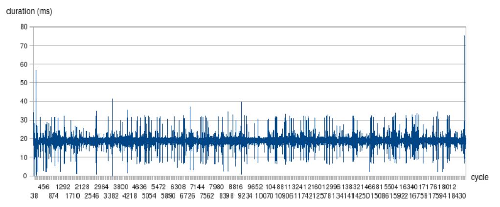
We realized that our agent's thread responsible for receiving messages from server sometimes took much more than the 20ms of server cycle (see figure 3). That made our agent receive message with some delay, in relation to the server, and thus lead it to mess up all movement planning. We then suspected of some lack of synchronization between our agent's threads, or within the server timer.
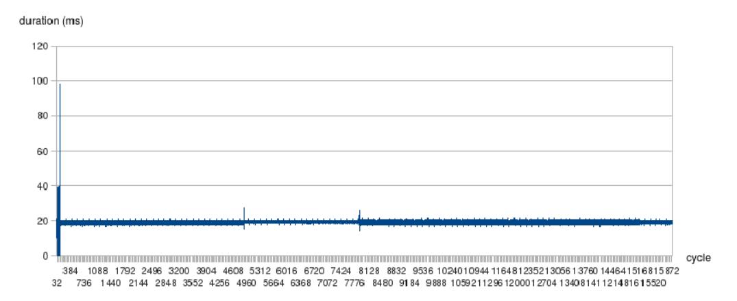
We reviewed the way our threads were synchronized, how is it that occurs synchronization between server and agents and improved our algorithms. Performance increased substantially (see figure 4), but now the situation has been reversed: when remotely connected the agent shows a great performance, while locally it's quite unstable. The computer machine involved still show performance interference, but without linear relation with higher processing capacity.
We are still trying to discover exactly what causes such instability when we connect our agents, specially through local connections. We expect a performance improvement after the new timer implemented on server (rcssserver3d 0.6.3), although we couldn't actually test it yet, due to ODE library and new server version conflicts within our machine server.
6 Results and Future Work
We obtained good results with our movement model, since our agent is now able to carry out with basic movements, such as walking, rising up and kicking, in a smooth and stable manner. Our next challenge, relating to movements, is to make them more flexible. For instance, turn the walk move so flexible we can choose step size and velocity during the match, in order to adapt to the most variable situations.
With basic movements implemented, we may step forward to implement high level decisions, taking into account game soccer strategies. And, due to our agents' architecture, gradually increment high level reasoning models will occur in a natural manner, since it was designed to accomplish that.
References
- van Dijk, S., Klomp, M., Neijt, B., Platje, M., van de Sanden, M.: Little green bats humanoid 3d simulation team description paper. In: Robocup Proceedings, Robocup (2008)
- Microsoft: Microsoft robotics studio. http://www.microsoft.com/Robotics/