Bahia3D Team Description Paper

Adailton J.C. Junior, Adriano V. Botelho, Ayran C. Cruz, Diego G. Frias Suarez, Josemar R. Souza, Marco A. C. Simoes, Murilo R. R. Alves

Bahia State University (ACSO/UNEB), Salvador, BA, Brazil

Abstract One of the major challenges in the development of a soccer playing team for RoboCup Simulation League 3D, for beginner groups, is embedding in the agents scripts with synchronized hinge angular velocities for moving the humanoid players in the desired way. For instance, make the Nao robot to walk as fast as possible in an stable way is not a quite simple task as it seems. In this paper we describe the new architecture of the agent of the Bahia3D team and our current approach for movement generation modeling. Additionally, we describe some works under development.

1 Introduction

Bahia3D is developed since 2009 by the Bahia Robotics Team (BRT) group, part of the Computer Architecture and Operating Systems group^1, that focus on investigating application of artificial intelligence methods on autonomous robots. BRT has been participating of other RoboCup leagues (Simulation 2D, Mixed Reality) since 2007, showing good results specially within Mixed Reality, in which it won third place at RoboCup 2009. In Robocup 2009 the Bahia3D team, based on Little Green Bats [1], had its first international competition achieving the 16th place in the league's overall ranking. Such approach was adopted since BRT had no prior experience with 3D basic challenges related with commanding and controlling the motion of the humanoid Nao robot [2].

After the 2009 competition, the Bahia3D team was completely programmed over new basis, mainly because the Little Green Bats was not updated for the new vision model in the simulated 3D league. The new agent architecture of the Bahia3D was published in the TDP of RoboCup 2010 [3]. All the basic movements of the agents of the 2010 team were adapted from logs obtained running Microsoft Robotic Studio (MSRS) [4] which provides an interface that simulates the Nao robot. The MSRS simulator has a set of predefined movements such as walking in different directions, stand up and turn around, among others, that can be executed writing a log file with the angles of all joints in each time interval of 0.02 seconds. Such data was used for building scripts with angular velocities of the hinges that were sent to 3D simulation league server Simspark [5] in order to reproduce such movements in the 3D competition environment. However, there was noise in the angular velocities obtained regardless of the approach used to approximate the discrete derivatives. After a careful smoothing of the time series of angular velocities, it was possible to make the Nao robot walk on the Simspark platform, even more stable and smooth than that observed in the MSRS simulator. Therefore, filtering high frequencies from the hinge angular velocity time series obtained from MSRS was worth it. Nevertheless, at Robocup 2010 our team was eliminated in the classificatory phase, loosing against very strong teams. In fact, the 2010 version of the Bahia3D team was extremely slow when compared with its state-of-the-art adversaries.

Thinking in Robocup 2011, the research group decided to improve the agent's basic skills. It was then implemented simple 2D kinematic models using two orthogonal coordinates: a longitudinal coordinate measured horizontally in the movement direction (forward or backward) and a vertical coordinate. The 2D kinematic models are run in scilab [6] generating scripts with angular velocities of the hinges participating in the movement. Such scripts in XML format are executed using an interface writen in C++ that starts a test-agent in the soccer-3D server. The movement of the Nao robot is monitored using Roboviz [7] and the sensors output is shown in real-time and compared with expected values according with the programmed movement. Such interface application, named IFAS3D, will be released soon when an stable version be ready.

This paper is structured as follows: In section 2, the bases of the kinematic model developed to simulate the robot's legs as he walks, are described. In section 3 the application interface used to test variations of moves in the same physical environment of the game, but without activating the game rules, is briefly shown. In section 4 the approach that is being tested for the agent to intercept the ball with higher efficiency is described. Finally in section 5 the conclusions of the work are drawn.

2 Kinematic 2D Model

The Agent Kinematic Module translates abstract actions received from the Brain module of our agent and into a proper command scripts. For instance, the Brain sends action "kick "and the Agent translates it into a specific command list to be executed in a finite number of time steps or server cycle, informing which joints are involved in such action and the corresponding angular velocities of each hinge during the action in order to perform the desired kick movement.

In the current state, the kinematic module has pre-built movement programs which are started according with the action sent by the Brain module. A program P is a nxm matrix with columns containing the program of the m hinges involved, which are comprised by the angular velocities of the hinges at each of the n cycles that the action should take. Angular velocities are placed consecutively in the rows of the program matrix P.

A generic executor routine receives the program matrix and builds the commands to be sent to the player, via the server. At each cycle the executor reads the corresponding row, and checks how the planned program has been executed until the current moment. In case of deviations found a feedback is included in the next command. In subsection 2.2 below, such feedback procedure is briefly described.

2.1 Construction of the Walking Program

A generic 2D kinematic model of a humanoid robot was used. Two orthogonal coordinates: a longitudinal (horizontal) axis in the movement direction and a vertical coordinate span the plane where the modeled Nao moves.

A simplified arm-less Nao scheme was built as shown in Figure 1. Eleven reference points are used for plotting the movement in scilab: head, shoulder, waist, right and left knees, ankles, tiptoes and heels, as indicated in the figure.

Fig. 1. Simplified Nao Scilab Geometrical Model

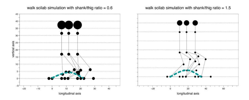
In order to make the model highly generic, most of the distances between those points are related with geometrical parameters. For example, given the thig length T, the shank length S is obtained by multiplying T by a given non-null positive parameter pST , in the form: S = pST T. Changing pST changes significantly the anatomy of the simulated humanoid robot as can be seen in Figure 2. In the same sense the size of the upper part of the robot U is related by a non-null positive parameter pUD to the size of the lower part S + T, in the form U = pUD(S + T). The distance from the waist to the shoulder, irrelevant in the studied case, is also set relative to the upper part size U.

In figure 2 the position of the reference points during the n cycles of a single step are plotted with overlapping. The driven event in the simulation is the forced displacement of one leg ahead describing a parameterized parabolic trajectory, while the opposite leg is kept fixed. Such simulated discrete trajectories of the reference points are then used to calculate the corresponding hinge angles series, from which the hinge angular velocities to be included in the movement program are calculated. A control of maximum achievable hinge rotation velocity is included to avoid unrealisitic programs.

2.2 Monitoring the Movement

As well as in the real environment, simulated environment also presents noises, so actions will not be always precisely executed. Therefore, to ensure previously described movement planning to be reasonably executed, we used the feedback method. The joint angles sent by the server are compared with the predicted values in the last two time steps (server cycles) with available data. The found deviation are used to predict the next deviation which is used in the calculation of the angular velocities to be sent to the server in the current time step. We used to forms of prediction of the next deviation: linear by extrapolation or by average. The agent selects the most proper form by monitoring the sign of the deviations. When it observes that the sign changes between time steps, the average prediction is chosen. Otherwise, the linear extrapolation.

If the deviation exceeds certain prefixed values during more than 10 cycles the agent turn off the feedback, because it is uneffective or perturbing in that situation. The moment and state variables when the feedback is turned off is registered in debug mode for further analysis.

3 Interface Application

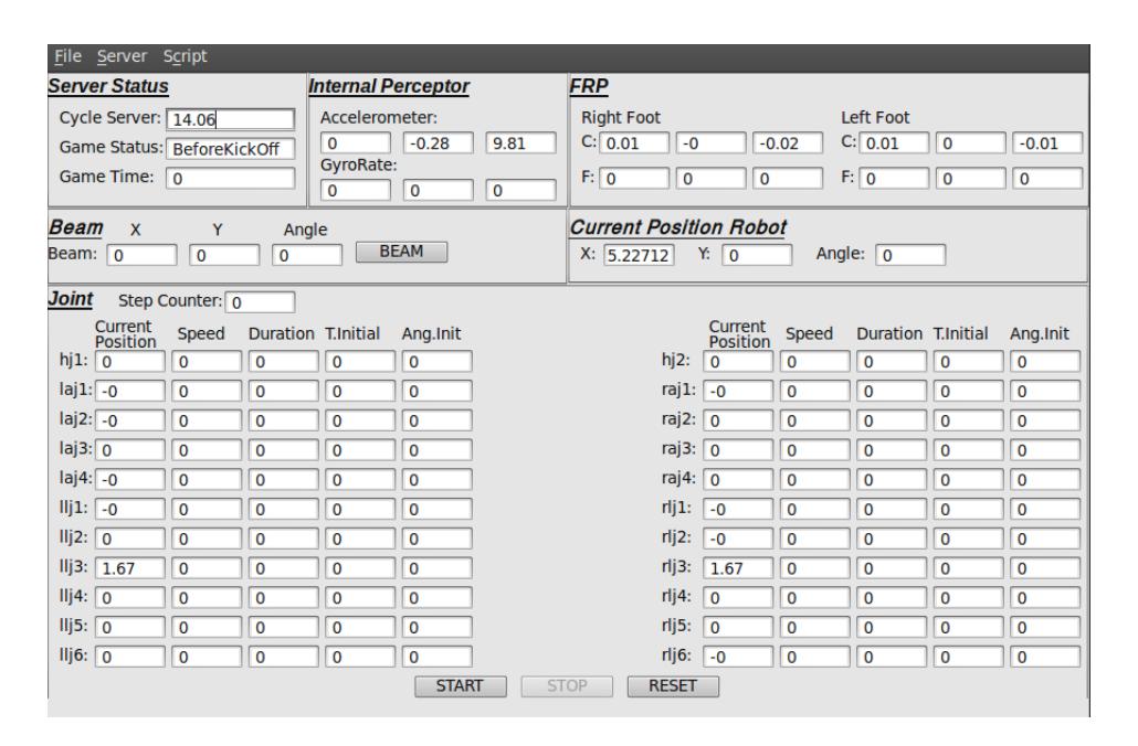
BRT group has developed an interactive interface application with Simspark, called IFAS3D, to visualize the response of the Nao robot to a sequence of commands that makes it to move synchronically a predefined set of hinges. One of the main attractive features of IFAS3D is that allows investigating the behavior of the robot without the interference of game rules and agent intelligence.

This tool establishes a connection with the Simspark simulator and creates a single agent in the actual version, which is placed in the desired position of the field using the command beam. IFAS3D allows the user to send hinge angular speeds time series and visualize, in real time, the resulting motion of the robot in the simulated environment. IFAS3D also allows saving the hinge rotation angles and speeds at each cycle which serves for further analysis.

Simple hinge angular speed time series can be set on the IFAS3D interface by setting constant angular velocities and the number of time cycles desired for each hinge. More complex time series can be read from input files in XML format.

4 Improving the Agent Ball Interception Capability

Once the robot can walk steady with three discrete speeds (slow, normal and fast) the Bahia3D team's major weakness is the lack of an algorithm for predicting the future position of the ball that allows the agent to plan the route necessary to intercept it, if the ball keeps the same state of motion. Currently, the reactive agent is scheduled to go directly to the direction of the ball, even if it is moving. In order to improve the agent ball interception capability the BRT group is now working on two parallel tasks: (1) improving Perception of Kinematic States (PKS) of both agent and ball, and (2) developing a Ball Interception Algorithm (BIA), which are described briefly in the next sections.

4.1 Improving Perception of Kinematic State

The 2D kinematic state of both agent and ball is comprised by 3 state variables: (1) position on the soccer field, $\mathbf{p}(t) = (p_x(t), p_y(t))$, (2) velocity, $\mathbf{v}(t) = (v_x(t), v_y(t))$ and (3) acceleration, $\mathbf{a}(t) = (a_x(t), a_y(t))$, where $t = \kappa \Delta t$ is a discrete time variable, that is, $\kappa = 0, 1, 2, \ldots$ and $\Delta t = 0.02$ seconds.

Our approach approximates current velocity and acceleration every time the current position $\mathbf{p}(\kappa^\Delta t)$ is calculated. Here $\kappa^$ denotes a current time cycle where it was possible to calculate the position from the data sent by the server, that is, using the approximated distances and angles to at least two visible flags on the field. Considering that the previous time cycle where the position $\mathbf{p}$ was updated is $\bar{\kappa}$, the current velocity is calculated as $\mathbf{v}(\kappa^\Delta t) = 1/\Delta t(\mathbf{p}(\kappa^\Delta t) - \mathbf{p}(\bar{\kappa}\Delta t))/(\kappa^* - \bar{\kappa})$ and the current acceleration as $\mathbf{a}(\kappa^\Delta t) = 1/\Delta t(\mathbf{v}(\kappa^\Delta t) - \mathbf{v}(\bar{\kappa}\Delta t))/(\kappa^* - \bar{\kappa})$.

Such estimated state variables are then used for predicting velocity and position until the next cycle when the position calculation will succeed, denote it by $\kappa^{\star\star}$. That is, for all $\kappa^{\star}<\kappa\leq\kappa^{\star\star}$ we predict $\mathbf{v}(\kappa\Delta t)=\mathbf{v}(\kappa^{\star}\Delta t)+\mathbf{a}(\kappa^{\star}\Delta t)(\kappa-\kappa^{\star})\Delta t$ and then $\mathbf{p}(\kappa\Delta t)=\mathbf{p}((\kappa-1)\Delta t)+\mathbf{v}(\kappa\Delta t)\Delta t$. The estimated position at $\kappa^{\star\star}$ helps in choosing between the two solutions for $\mathbf{p}$ obtained by triangulation with two visible flags. This simple approach improved significantly the accuracy of the Bahia3D agent as compared with the 2010 version.

Taking into account that every three time cycles (0.06s) the server sends data for updating the kinematic states of agent and ball, even that if in some of such opportunities the agent localization did not succeed, such kind of prediction is done during a very short time interval, why we called it as short-range prediction. Large range prediction of ball state is implemented in the ball interception algorithm described in the next section.

4.2 Ball Interceptation Algorithm

The first calculation in the ball interception algorithm is the estimation of the ball current position on the filed b, having the agent current position p. This is done into three steps: (1) calculate the entries of a unitary vector c on the head of the robot co-linear with the camera using the angle between the camera and one of the two flags used for triangulation, (2) rotate c until pointing towards the ball using the angle-to-ball provided by the server, and (3) expands c multiplying by the distance-to-ball provided by the server and add the agent position vector p.

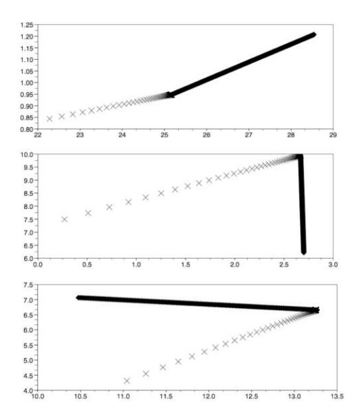
Thereafter, the velocity of the ball s is estimated as described above and a large range prediction procedure is started. This procedure assumes a continuous slowing down at each time cycle, in the form s(κ∆t) = φ s((κ − 1)∆t), where 0 < φ ≤ 1 takes into account the lost of kinetic energy by friction and is expected to be adjusted automatically by the agent using predicted ball velocities b in several times steps. This way the ball position prediction accuracy will not depend on the Open Dynamics Engine (ODE) configuration.

5 Concluding Remarks

In the last year the Bahia3D team have evolved significantly as compared with the previous two versions. In particular, the generation of a walking program based on a theoretical and highly parameterized kinematic model allowed the robot to walk stably with an approximate speed of one feet per second and will support further improvements.

Using IFAS3D it was possible to reduce the overall time of the study, allowing us to isolate the robot from the game environment, turning off his intelligence and focusing on the analysis of the kinematics of the motion for the several walking programs under test. The authors hope that this tool might help other beginner 3D teams and are working hard for releasing an stable version before June 2011.

Regarding the improvement of the perception (acquisition) by the agent of the kinematic information (position, vectorial velocities and acelerations) of the robot itself and of the ball, as well as, regarding the efficacy of the ball interception algorithm in real conditions, we have not yet conclusive results. However, the preliminary results (not shown) are promissory.

The next step will be focused on improving the intelligence of the agent in order to have a highly competitive team in 2012.

References

1. van Dijk, S., Klomp, M., Neijt, B., Platje, M., van de Sanden, M.: Little green bats humanoid 3d simulation team description paper. In: Robocup Proceedings, Robocup (2008)
2. Aldebaran: Aldebaran robotics. http://www.aldebaran-robotics.com/
3. de J. Cerqueira Jr., A., Botelho, A.V., Frias, D., oes, M.A.C.S., Souza, J.R.: Bahia3d a team of 3d simulation for robocup. In: Robocup Proceedings. (2010)
4. Microsoft: Microsoft robotics studio. http://www.microsoft.com/Robotics/
5. SimSpark: Simspark wiki. http://simspark.sourceforge.net/wiki/
6. Scilab: Scilab home page. http://www.scilab.org/
7. Roboviz: Roboviz home page. https://sites.google.com/site/umroboviz/
8. Qt: Qt a cross-platform application and ui framework. http://qt.nokia.com/