Mithras3D Team Description Paper 2014 Soccer Simulation 3D League

Armita Sabeti Ashraf, Atieh Alsadat Moosavian, Fatemeh Gerami Gohar, Fatima Tafazzoli Shadpour, Romina Moradi, Sama Moayeri

Farzanegan (1) High school, Tehran, Iran

Abstract In this paper we describe Farzanegan soccer simulation team activities. After an introduction to the Soccer Simulation 3D League we will describe our team architecture and its behavior which contains some skills used in order to deal with several challenging problems in this field such as balancing, movements, making decision.

Keywords: Inverse and Forward Kinematic, Modeling, Denavit Hartenberg.

1 Introduction

Farzanegan High school Laboratory has been working on RoboCup science for many years and achieved many remarkable successes in different Robocup Competition Leagues. Our simulation group had been working on Rescue Simulation League, Soccer Simulation 2D League and subsequent to this our researches has been started in Soccer Simulation 3D since 2009.

The RoboCup 3D Simulated Soccer League allows software agents to control humanoid robots to compete against one another in a realistic simulation of the rules and physics of a game of soccer. The platform strives to reproduce the software programming challenges faced when building real physical robots for this purpose. The Robocup simulation leagues focus on AI and team strategies developed by the participant teams. The 3D simulation competition increases the realism of the simulation environment by adding an extra dimension and more complex physics. The interest in the 3D simulation competition is design of implementation of Multi-agent high-level behaviors.

2 Team Architecture

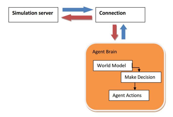
The base code was written in 2009, and after that our development and optimization activities has been started on it. Classify agent behavioral layers which exist in base code help us to design some methods to make good decisions.

• Simulation Server
• Connection
• Agent Brain
• World Model
• Make Decision
• Agent Actions

2.1 Connection

This class is responsible for communicating with server. It synchronizes different threads of execution with server timing. When the new information arrives, the connection layer updates the agents WorldModel.

2.2 Command

This class makes the commands which we send to the server.

2.3 Mathematics

Here are our mathematical classes such as Vector and Matrix.

2.4 Utilities

In this folder we have some useful classes such as config (which we use in order to initialize some variables and change them easily.) converter (which we use in order to convert different types of values to each other, for example degree to radian or Cartesian coordinate system to spherical coordinate system.) Logger, Timer and Types.

2.5 Kinematics

Here we have the Forward and Inverse Kinematic classes which will be explained later.

2.6 WorldModel

Worldmodel contains main and basic calculations used in actions of robot like walking, turning and decision. In this part we are dealing with position and rotation status of each object on the field. And of Course for the agent itself, we calculate useful information about joints of agent, forces which are applied towards it, gyroscope, etc. In each cycle, server sends a string of information with specific format and arrangement. First of all, we make a graph out of information that server sends. After that, in each cycle of time, we extract the information and update our model of world. Some information follows simple form of updating. For example, to update angle of turning we just specify, individualize and then save raw data. But for updating vector of accelerometer and amounts of gyroscope, we need some calculations. Server gives amount of changes in accelerometer vector since last time, but we need accelerometer vector itself. So we do one integral on it. More complicated calculations are in localization of agents and ball. To check whether robot is falling down or not or calculate the angle between agent and any point in field, we save information that server gives us in each cycle and use complicated calculations. For example, raw information received from server contains seen objects by robot, the way it sees them. Its moves and turns in neck joints and body situations influence the numbers. So the first thing to do is to turn those relative positions to universal positions using rotation matrixes which rotates back all those relative positions. Since neck turn does not depend on body rotation, we need different matrixes, neck and body. Neck rotation matrix is calculated easily since it is consist of two simple joints and we have the angles. But the body rotation matrix is somehow more complicated. We briefly say that it can be calculated in two different ways, in the first way we use gyroscope preceptor and in the second one we use relative information from horizontal and vertical lines on the field.

After doing calculations we have different position of the robot with low disagreement. For finding the correct position of the robot we use weighted average on the whereabout position.

2.7 Agent

The agents must contain some procedures which manage their behaviors. Robot needs special skills to play better, such as kick, pass, dive, stand up (which itself has different kinds depended on the way that the agent falls. Standup from front, back, left side or right side), turn (rotates to place where is asked). These skills are written in this part. This part is divided in to some layers in order to be more organized. The Inheritance of Agent class is shown below:

• Joint Controller
• Body Controller
• Robot
• Basic Agent
• Agent
• Advanced Agent
• Our Player

3 Walking

we implemented walking with repeating stable steps. Each step is divided into two movements: raising the leg and moving it forward, and then taking it down during moving it forward again.

The magnitude of upward and forward motion is optimized by utilizing PSO algorithm. [5]

We used Inverse Kinematics to commute these magnitudes into proper values for the joint angles, which are given as inputs to the motion functions.

Inverse Kinematic is a method to compute a set of joint angles that satisfy the end-effecter constrains.

For stability some physical factors must be considered. One of these factors is Center of Mass (CoM). We can also use other dynamic feedbacks such as Zero Moment Point (ZMP). In stable patterns this point must be within the supporting area. (The convex hull of the robot's feet.)

3.1 Forward Kinematic

Our purpose in this algorithm is determining the position of the joints and other points with knowing the angles of the joints.[2] One of the methods which helps us to achieve this purpose is Denavit Hartenberg.[3] In fact, this method goes from joint to joint in four steps, multiplying a matrix in the previous matrixes in each step.

1 st Step: a displacement along Z axis

2 nd Step: rotation around Z axis

3 rd Step: displacement along X and Y axes

4 th Step: rotation around X axis

After going joint to joint, the final matrix must be multiplied by the inverse of the total rotation matrix in order to obtain the coordinates in the universal coordinate system.

 \begin{aligned} & \textbf{Matrixform} \\ & \textbf{Chop} [\textbf{rallEinplify}] \begin{bmatrix} \cos(-\alpha_1) - \sin(-\alpha_1) & 0 & 0 \\ \sin(-\alpha_1) - \cos(-\alpha_1) & 0 & 0 \\ 0 & 0 & 1 \end{bmatrix} \begin{bmatrix} 1 & 0 & 0 & -0 & 0 \\ 0 & 0 & 1 & 0 \\ 0 & 0 & 1 \end{bmatrix} \begin{bmatrix} 1 & 0 & 0 & -0 & 0 \\ 0 & 0 & 1 \\ 0 & 0 & 0 \end{bmatrix} \begin{bmatrix} 1 & 0 & 0 & -0 & 0 \\ 0 & 0 & 1 \\ 0 & 0 & 0 \end{bmatrix} \begin{bmatrix} 1 & 0 & 0 & -0 & 0 \\ 0 & 0 & 1 \\ 0 & 0 & 0 \end{bmatrix} \begin{bmatrix} 1 & 0 & 0 & -0 & 0 \\ 0 & 0 & 1 \\ 0 & 0 & 0 \end{bmatrix} \begin{bmatrix} 1 & 0 & 0 & -0 & 0 \\ 0 & 0 & 1 \\ 0 & 0 & 0 \end{bmatrix} \begin{bmatrix} 1 & 0 & 0 & -0 & 0 \\ 0 & 0 & 1 \\ 0 & 0 & 0 \end{bmatrix} \begin{bmatrix} 1 & 0 & 0 & -0 & 0 \\ 0 & 0 & 1 \\ 0 & 0 & 0 \end{bmatrix} \begin{bmatrix} 1 & 0 & 0 & -0 & 0 \\ 0 & 0 & 1 \\ 0 & 0 & 0 \end{bmatrix} \begin{bmatrix} 1 & 0 & 0 & -0 & 0 \\ 0 & 0 & 1 \\ 0 & 0 & 0 \end{bmatrix} \begin{bmatrix} 1 & 0 & 0 & -0 & 0 \\ 0 & 0 & 1 \\ 0 & 0 & 0 \end{bmatrix} \begin{bmatrix} 1 & 0 & 0 & -0 & 0 \\ 0 & 0 & 1 \\ 0 & 0 & 0 \end{bmatrix} \begin{bmatrix} 1 & 0 & 0 & -0 & 0 \\ 0 & 0 & 1 \\ 0 & 0 & 0 \end{bmatrix} \begin{bmatrix} 0 & 0 & -0 & 0 \\ 0 & 0 & 0 \end{bmatrix} \begin{bmatrix} 0 & 0 & -0 & 0 \\ 0 & 0 & 0 \end{bmatrix} \begin{bmatrix} 0 & 0 & -0 & 0 \\ 0 & 0 & 0 \end{bmatrix} \begin{bmatrix} 0 & 0 & -0 & 0 \\ 0 & 0 & 0 \end{bmatrix} \begin{bmatrix} 0 & 0 & -0 & 0 \\ 0 & 0 & 0 \end{bmatrix} \begin{bmatrix} 0 & 0 & -0 & 0 \\ 0 & 0 & 0 \end{bmatrix} \begin{bmatrix} 0 & 0 & 0 \\ 0 & 0 & 0 \end{bmatrix} \begin{bmatrix} 0 & 0 & 0 \\ 0 & 0 & 0 \end{bmatrix} \begin{bmatrix} 0 & 0 & 0 \\ 0 & 0 & 0 \end{bmatrix} \begin{bmatrix} 0 & 0 & 0 \\ 0 & 0 & 0 \end{bmatrix} \begin{bmatrix} 0 & 0 & 0 \\ 0 & 0 & 0 \end{bmatrix} \begin{bmatrix} 0 & 0 & 0 \\ 0 & 0 & 0 \end{bmatrix} \begin{bmatrix} 0 & 0 & 0 \\ 0 & 0 & 0 \end{bmatrix} \begin{bmatrix} 0 & 0 & 0 \\ 0 & 0 & 0 \end{bmatrix} \begin{bmatrix} 0 & 0 & 0 \\ 0 & 0 & 0 \end{bmatrix} \begin{bmatrix} 0 & 0 & 0 \\ 0 & 0 & 0 \end{bmatrix} \begin{bmatrix} 0 & 0 & 0 \\ 0 & 0 & 0 \end{bmatrix} \begin{bmatrix} 0 & 0 & 0 \\ 0 & 0 & 0 \end{bmatrix} \begin{bmatrix} 0 & 0 & 0 \\ 0 & 0 & 0 \end{bmatrix} \begin{bmatrix} 0 & 0 & 0 \\ 0 & 0 & 0 \end{bmatrix} \begin{bmatrix} 0 & 0 & 0 \\ 0 & 0 & 0 \end{bmatrix} \begin{bmatrix} 0 & 0 & 0 \\ 0 & 0 & 0 \end{bmatrix} \begin{bmatrix} 0 & 0 & 0 \\ 0 & 0 & 0 \end{bmatrix} \begin{bmatrix} 0 & 0 & 0 \\ 0 & 0 & 0 \end{bmatrix} \begin{bmatrix} 0 & 0 & 0 \\ 0 & 0 & 0 \end{bmatrix} \begin{bmatrix} 0 & 0 & 0 \\ 0 & 0 & 0 \end{bmatrix} \begin{bmatrix} 0 & 0 & 0 \\ 0 & 0 & 0 \end{bmatrix} \begin{bmatrix} 0 & 0 & 0 \\ 0 & 0 & 0 \end{bmatrix} \begin{bmatrix} 0 & 0 & 0 \\ 0 & 0 & 0 \end{bmatrix} \begin{bmatrix} 0 & 0 & 0 \\ 0 & 0 & 0 \end{bmatrix} \begin{bmatrix} 0 & 0 & 0 \\ 0 & 0 & 0 \end{bmatrix} \begin{bmatrix} 0 & 0 & 0 \\ 0 & 0 & 0 \end{bmatrix} \begin{bmatrix} 0 & 0 & 0 \\ 0 & 0 & 0 \end{bmatrix} \begin{bmatrix} 0 & 0 & 0 \\ 0 & 0 & 0 \end{bmatrix} \begin{bmatrix} 0 & 0 & 0 \\ 0 & 0 & 0 \end{bmatrix} \begin{bmatrix} 0 & 0 & 0 \\ 0 & 0 & 0 \end{bmatrix} \begin{bmatrix} 0 & 0 & 0 \\ 0 & 0 & 0 \end{bmatrix} \begin{bmatrix} 0 & 0 & 0 \\ 0 & 0 & 0 \end{bmatrix}

Fig. 3. matrix chain for moving from torso to the right sole

3.2 CoM(Center of Mass)

We used the forward Kinematic method to find the centers of the bodies of the Nao robot (for example each hand itself has two bodies, and each Leg itself has three bodies.). Then we can compute Center of mass of the whole robot with this formula:

$$\frac{\sum m_i * p_i}{\sum m_i}$$

When $m_i$ is mass of the body and $p_i$ is the position of the center of the body.

3.3 Inverse Kinematic

Robot control actions are executed in the joint coordinates while robot motions are specified in the Cartesian coordinates. Conversion of the position and orientation of a robot from Cartesian space to joint space, called as inverse kinematics problem, which is of fundamental importance in calculating desired joint angles for robot design and control.

The algorithm uses the displacements of each joint then gives us joint angles. For a robot with n degree of freedom, at any instant of time joint variables is denoted by $\theta_i = \theta_{(t)}, i = 1, 2, \dots, n$ , and position variables $X_i = X_{(t)}, i = 1, 2, \dots, n$ . The relations between the position $X_{(t)}$ and joint angle $\theta_{(t)}$ can be represented by forward kinematic equation, $X_{(t)} = f(\theta_{(t)})$ .

The Inverse Kinematic exactly does the visa versa thing, it means that it gets the position and produces the appropriate angles.

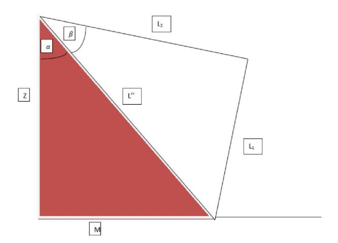
At first we had simplified the problem with some assumptions. For example we have omitted the first joint in our calculation temporarily and will add it later. And we tried to have the ankle parallel to the ground. So we find these equations:

$$\alpha = \arctan(\frac{M}{Z})$$

$$\beta = \arccos(\frac{l_1^2 - l_2^2 - l_1^{2}}{-2l_2*l})$$

$$\theta_3 = \alpha + \beta$$

$$\theta_4 = -\arccos(\frac{l_1^* - l_2^2 - l_2^2}{-2l_1l_2} + 180)$$

$$\theta_5 = -\theta_3 - \theta_4$$

$$\theta_2 = -\arctan(\frac{Y}{Z})$$

$$\theta_6 = -\theta_2$$

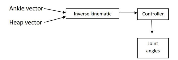
Nao is a humanoid robot with 6 DoF (Degrees of Freedom) in each leg. Joints 1, 2 and 3 are in the same place and joints 5 and 6 are in another same place .We use heap vector as the place of joints 1, 2 and 3 and ankle vector as the place of joints 5 and 6 to solve inverse kinematic equations. Then we check equppations answer for confidence that whether the answers produced are in the limited operating or not. Therefore, use Inverse kinematics formula for determining joint angles for each joint. This is implemented as a periodic state machine.

Befor now we couldn't calculate the first engine with our IK equations. But we changed the Idea and now we can commute the first engine too. We've found a relation between the first engine value and the rotation of Ankle around Zaxes, So we use the proper rotation for this engine. Then we change the frame of solving the problem by knowing this value and using forward kinematic methods and then we find the exact value of other engines.

Actually we have calculated the jacobian matrix and we have implemented the IK with using jacobian based methods such as iterative ones. But we are testing both of this methods to find which one is better.

4 Online Modeling

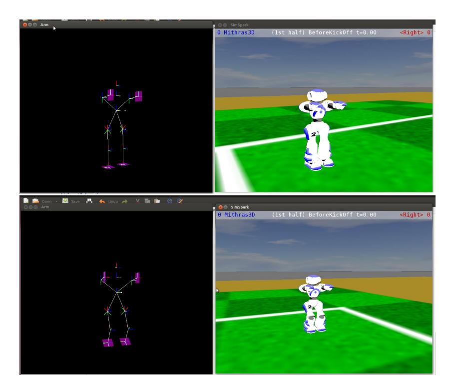
In order to observe the robot actions better we have modeled the Nao robot in OpenGL which works parallel to the Simspark server with getting some outputs from the agent.

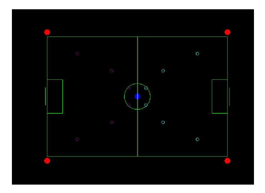
And also in order to observe the worldmodel calculations we modeled the ground as a 2dmonitor in OpenGL.

5 Future Works

In the worldmodel part we are working on minimizing the errors. In order to do this we want to add some filters to our calculates.

And also we are optimizing the skills and decision making of the Agent. We are working to use the CoM that we have calculated in order to make more stable motions.

References

1. Atieh AlSadat Moosavian , Sara Javadzadeh No , Armita Sabeti Ashraf ,Nazanin Sadat Dastserri, Farzanegan Team Description Paper 2011 Soccer Simulation 3D league
2. http://www.cs.duke.edu/brd/Teaching/Bio/asmb/current/Papers/chap3-forwardkinematics.pdf
3. Ravi Balasubramanian, The Denavit Hartenberg Convention
4. Rcssserver3d user manual
5. Cord Niehaus, Thomas Rofer , Tim Laue, "Gait Optimization on Humanoid Robot using Particle Swarm Optimization".
6. Joao Certo,Nuno Lau, Lus Paul Reis, "Multi-Agent Coordination through Strategy"
7. http://www.wikipedia.org/