ITAndroids Soccer3D Team Description Paper 2017

Dicksiano Melo, Eric Endo Soares, Eric Moreira, Francisco Muniz, Guilherme Marra, Gustavo Nahum, Helúdio Lopes, José Lucas Saraiva, José Otávio Vidal, Juan Freire, Luckeciano Melo, Marcos Maximo

Aeronautics Institute of Technology, São José dos Campos, São Paulo, Brazil

http://www.itandroids.com.br/pt-BR

Abstract ITAndroids was reestablished in mid-2011 by undergraduate students at Aeronautics Institute of Technology. Since then, the team is growing fast and has already established itself as a strong robotics competition group, winning several competitions in Brazil and Latin America.

1 Introduction

ITAndroids is a robotics competition group associated to the Autonomous Computational Systems Lab (LAB-SCA) at Aeronautics Institute of Technology. As required by a complete endeavor in robotics, the group is multidisciplinary and contains about 40 students from different undergraduate engineering courses. In the last 5 years, we have achieved good results in competitions, especially in Latin America.

Our older Soccer 3D team had a Base made from Magma Offenburg, but since RoboCup 2016 we use our own Base using C++. Currently, ITAndroids is the only team of Latin America which uses its own Base code. RoboCup 2016 was the first run and we achieved the 6th place.

This paper describes our development efforts in the last years and points out some improvements we want to implement in a near future. Sec. 2 describes our team's code structure. In Sec. 3, we discuss our localization method. In Sec. 4, we show our motion control system. Sec. 5 explains our role assignment system for positioning. Sec. 6 shows our strategy and points our robot navigation method. Finally, Sec. 7 concludes and shares our ideas for future work.

2 Code Structure

The code has been planned and divided in several modularized parts, so that each part can be separated from the others with ease. ITAndroids Soccer 3D used to work with a Base made from Magma Offenburg and ITAndroids Soccer 2D works with Agent2D. In this way, our current code structure was heavily influenced by those works.

2.1 Communication

It is the layer that directly connects with the server, in order to receive messages and send messages to it. This layer receives and sends a string as described in the server's website. It uses a socket to implement the communication, receiving a message that contains the information from the server.

2.2 Perception

This layer receives the string from Communication, and converts the string into a tree, parsing it. The layer then iterates over the created tree and creates new objects from it, so that the agent can have new information each new loop. The created objects come in the form of perceptors and each perceptor is as described in the server's website.

2.3 Modeling

Modeling basically models the world state. Not only that, it also models situations, e.g. in whether the agent has fallen. It uses the perceptors created in perception to update its models, getting the relative position of field landmarks to find it's positions, and acelerometer data to see if the agent has fallen.

Agent Model

The Agent model is the part of the code that models specific agent modes. It calculates the transformation matrices, in order to change the coordinate system from the camera to a ground coordinate system, using robot joints and making simplifications on the system.

World Model

The World Model is responsible for modeling parameters like game state, time, and position, so that these information can be used by Decision Making. It runs the Localization algorithm in order to estimate the robot's position.

2.4 Decision Making

Decision Making is a layer that divides each robot by decision makers. It consists Behavior and Decision Maker. One agent cannot change its decision maker, but, that decision maker must be able to integrate all the possible behavior the agent has available, e.g. a Soccer agent receives a SoccerDecisionMaker, and a goalie receives a GoalieDecisionMaker. Those decision makers dictate the movements the agent should take in order to successfully follow a determined strategy.

Behavior is a set of what the agent can to in order to change its own state. Behavior is a set of instructions that goes from high to low level of abstraction, in order to make the agent follow it's strategy. Each behavior can use other behaviors for a more abstract level of problem solving.

The layer has two parts, a part that is a data structure called BehaviorFactory, and a structure called Behavior. A BehaviorFactory stores all behaviors within itself, and each behavior has access to all other behaviors in the Behavior Factory.

2.5 Control

Control is the layer that gets the requests from behavior and changes it into more concrete things. For example, it takes a walk request created from one of the behaviors, and converts it into joints positions.

2.6 Action

Action is a layer that converts all the information the agent has created and wants to send to the server into a string, in a way the server can recognize.

3 Localization

Using complex strategies in robot soccer requires that the agent knows its global position in the soccer field. The problem of having a mobile robot estimates its pose with respect to a global coordinates system is termed Localization in the robotics community. To solve this problem, the standard approach involves using a Bayes filter, which iteratively incorporates sensors' measurements and the robot's actions to construct a probabilistic estimate of the robot position. Since implementing this technique directly is not feasible computationally, approximated techniques, such as the Kalman filter [9] or the particle filter [10], are often employed. We decided to use Monte Carlo localization (MCL) [5], which uses a particle filter to solve the Localization problem, because it is one the most efficient methods [8] and some teams in 3D Soccer Simulation have successfully used this technique [3, 4].

Our MCL implementation was greatly inspired by the work explained in [6]. Each particle mantains a pose estimate represented by a 3-dimensional vector $\mathbf{x} = [x, y, \psi]^T$, where x and y are global field coordinates and $\psi$ is the horizontal angle the torso of the robot is heading. We use a bootstrap particle filter with resampling step [11].

In the sensing phase, we currently landmarks (flags and goalposts) observations and line observations. Our landmark observation model consider gaussian noises corrupting the horizontal distance and horizontal angle measurements with covariances $\sigma_d^2$ and $\sigma_\psi^2$, respectively. Furthermore, we consider that landmarks observations are independent of each other. Therefore, a suitable rule for updating the particles' weights is:

$$w_k^{(i)} = w_{k-1}^{(i)} \prod_j \left{ \exp\left[ -\left(\frac{d_j - \hat{d}_j^{(i)}}{\sigma_d}\right)^2 \right] \cdot \exp\left[ -\left(\frac{\psi_j - \hat{\psi}j^{(i)}}{\sigma\theta}\right)^2 \right] \right}$$

where $w_k^{(i)}$ is the weight of the i-th particle in the k-th sampling time, $d_j$ is the measured horizontal distance between the robot and the j-th landmark, $d_j^{(i)}$ is the horizontal distance between the robot and the j-th landmark considering the current i-th particle's position, $\hat{\psi}j^{(i)}$ is the measured horizontal angle between the j-th landmark and the robot's heading, $\psi_j^{(i)}$ is the expected horizontal angle between the j-th landmark and the robot given the i-th particle position. To determine adequate values for $\sigma_d$ and $\sigma\psi$, we started with measurement covariances presented in Simspark's documentation and finely tuned these values by hand. We do not execute a sensing phase when no vision update is present (note that Simspark sends vision updates only every 3 cycles).

For motion update, we use odometry information given by our walking engine, which gives the torso displacement vector $\Delta \mathbf{d}_k = \left[\Delta x_k, \Delta y_k, \Delta \psi_k\right]^T$ relative to the local torso coordinates frame of the previous time step. At first, slipping was making odometry and actual movement differ too much, especially at high walking speeds. Simply scaling each channel proved effectively in solving this:

$$\mathbf{d}{k}' = \begin{bmatrix} \Delta x{k}' \ \Delta y_{k}' \ \Delta \psi_{k}' \end{bmatrix} = \begin{bmatrix} \alpha \Delta x_{k} \ \beta \Delta y_{k} \ \gamma \Delta \psi_{k} \end{bmatrix}$$

Thus, $\mathbf{d}'$ was the value of displacement effectively used for motion update. The parameters $\alpha$, $\beta$ and $\gamma$ were manually tuned by comparing the evolution of the robot's position and its estimate in Roboviz while the robot was walking. relative to the robot's coordinates frame) and manually tweaking $\alpha$, $\beta$ and $\gamma$. Then, we update the position of each particle i using:

$$\mathbf{x}{k} = \begin{bmatrix} x{k}^{(i)} \ y_{k}^{(i)} \ \psi_{k}^{(i)} \end{bmatrix} = \begin{bmatrix} x_{k-1}^{(i)} + \Delta x_{k}' \cos(\psi_{k-1}) - \Delta y_{k}' \sin(\psi_{k-1}) \ y_{k-1}^{(i)} + \Delta x_{k}' \sin(\psi_{k-1}) - \Delta y_{k}' \cos(\psi_{k-1}) \ \psi_{k-1}^{(i)} + \Delta \psi_{k}' \end{bmatrix} + \begin{bmatrix} \varepsilon_{x} \ \varepsilon_{y} \ \varepsilon_{\psi} \end{bmatrix}$$

where $\varepsilon_x \sim \mathcal{N}\left(0, \sigma_x^2\right)$, $\varepsilon_y \sim \mathcal{N}\left(0, \sigma_y^2\right)$ and $\varepsilon_\psi \sim \mathcal{N}\left(0, \sigma_\psi^2\right)$ incorporate process noise. These covariances were also manually tweaked. We execute a motion phase every cycle, then we naturally run more motion than sensing phases.

To reduce particle deprivation, we use a resampling step after sensing and motion phases [11]. Given that resampling algorithms may be computationally expensive, we use the O(N) algorithm shown in [8], where N is the number of particles used.

To avoid the kidnapped robot problem, which happens in the 3D Soccer Simulation domain when the server teleports the agent, we used the strategy known as Adaptive-MCL [7, 8], which resets particles based on a heuristic estimate of how bad localized the agent is. Instead of distributing the resetted particles randomly in the soccer field [6], we use the current vision observations to better reset the particles [7].

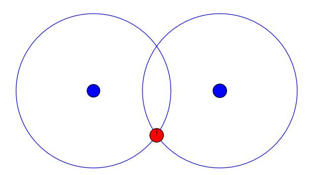
Given that two landmarks observations, we may estimate where the robot is as shown in Figure 1. Note that we end with two hypotheses, which may be chosen at random. In our case, one of them will usually falls outside of the soccer field, thus may be discarded. If more than two landmarks are seen in the current cycle, two landmarks are chosen at random for each particle which is being resetted. Moreover, we add gaussian noises to the landmarks' observations before applying this resetting process to better spread the resetted particles.

Finally, the agent's position estimate is determined by a weighted average of the particles' positions. For future work, we expect to determine the parameters using experiments or optimization techniques instead of relying on manual tweaking.

Fig. 1. Determining the agent's localization using two landmarks observation.

4 Motion Control

In 3D Soccer Simulation league, most actions of the robots are highly dependent on its ability to walk. Therefore, a great amount of our team efforts was focused on walking. In order to end a good walking method, several ideas were tested. Our latest walking models are described in this section.

4.1 ZMP Based Omnidirectional Walking Engine

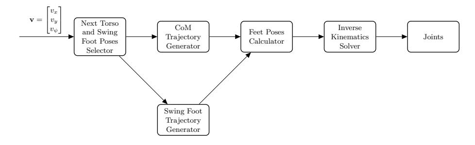
In general terms, the walking engine follows the flux presented on Figure 2. The input to the algorithm is the desired velocity v = [vx, vy, vψ]^T with respect to the local coordinate system of the robot. Then, at the beginning of a new step, poses for the torso and the swing foot are selected for achieving the expected displacement at the end of the step. So, a trajectory for the center of mass (CoM) that keeps the Zero Moment Point (ZMP) at the center of the support foot is computed by using an analytic solution of the 3D-LIPM equation. We approximate the CoM by a fixed position in the torso. The trajectory of the swing foot is obtained by interpolating between the initial and final poses of this foot. Finally, joints angles are calculated through Inverse Kinematics (IK) considering the poses of the support and swing feet. Note that the module "Next Torso and Swing Poses Selector" is called once for step, while the others are executed at the update rate of the joints.

A humanoid robot must satisfy dynamical constraints to remain stable. Moreover, the robot geometry imposes constraints: leg reachability is limited by leg physical dimensions and we also do not want movements where the legs collide. To achieve dynamic stability, our strategy is to generate a CoM trajectory that keeps the ZMP at the center of the support foot during single support. We may at least restrict the initial and final positions of this CoM trajectory, as will be explained below. Hence, our requirement is to have the robot matches the omnidirectional model only at the beginning and at the end of the step. Assuming constant v, we may compute the expected pose after a step duration T:

$$\begin{bmatrix} x[k+1] \ y[k+1] \ \psi[k+1] \end{bmatrix} = \begin{bmatrix} x[k] + 2\frac{v_x}{v_\psi} \sin\left(\frac{v_\psi T}{2}\right) \cos\left(\psi[k] + \frac{v_\psi T}{2}\right) - 2\frac{v_y}{v_\psi} \sin\left(\frac{v_\psi T}{2}\right) \sin\left(\psi[k] + \frac{v_\psi T}{2}\right) \ y[k] + 2\frac{v_x}{v_\psi} \sin\left(\frac{v_\psi T}{2}\right) \sin\left(\psi[k] + \frac{v_\psi T}{2}\right) + 2\frac{v_y}{v_\psi} \sin\left(\frac{v_\psi T}{2}\right) \cos\left(\psi[k] + \frac{v_\psi T}{2}\right) \ \psi[k] + v_\psi T \end{bmatrix}$$

For our multibody humanoid robot, it is convenient to select a body part as representative of the whole robot motion: we choose the torso for this. Thus, at the beginning of a new step, given the current torso and swing foot poses, an algorithm plans the torso and swing foot poses at the end of the step to make the torso arrive at the pose dictated by Equation (4) while trying to satisfy geometric constraints. This algorithm is based mainly on heuristics.

We still need to move the robot without losing balance. To reason about the robot dynamics, we approximate it using the 3D Linear Inverted Pendulum Model (3D-LIPM) [1]:

$$\mathbf{x}{ZMP} = \mathbf{x}{CoM} - \frac{z_{CoM}}{g} \ddot{\mathbf{x}}_{CoM}$$

Where xZMP = [xZMP , yZMP ]^T is the ZMP position, xCoM = [xCoM, yCoM]^T is the CoM position, zCoM is the CoM height, and g is the acceleration of gravity. The ZMP is kept at the center of the support foot during single support and moves it from the current support foot to the next one during double support.

However, the difference between the multibody humanoid robot dynamics and 3D-LIPM and perturbations, such as external forces and uneven terrain, will prevent the ZMP to match the reference. The robot is able to accommodate ZMP error up to the margins of the support polygon without tipping, which is often suffcient to allow open-loop walking if no strong perturbations are present. Nevertheless, closed-loop balancing strategies are useful to make the walking more robust. We have tried using the angular velocities measured from the gyrometer to stabilize the walk, which proved effective.

4.2 Kick

We consider that kicking is a motion where the biped starts in a stand position, kicks the ball and returns to the same stand position. Moreover, during kicking, one foot is taken off the ground, henceforth referred as kicking foot, while the other one is kept on the ground as support foot. This description suggests breaking the motion in phases, thus we divided it in the following 5 phases:

Phase A: the robot moves the ZMP to the center of the support foot to allow the kicking foot to be taken off the ground in the next phase without balance loss.
Phase B: the robot takes the foot off the ground and position it to prepare for kicking the ball.
Phase C: the robot kicks the ball.
Phase D: the robot places the kicking foot on the ground.
Phase E: the robot goes back to the stand position (ZMP is moved to the torso projection on the ground).

During phases B, C and D, the robot is in single support, so stability is of concern. Based on this perception, we use the same algorithm we used to balance walking for balancing kicking. Again, we constraint the CoM to maintain a constant height zCoM, so the dynamics becomes linear.

4.3 Keyframe Movement

A Keyframe movement is a movement where the positions of the joints are defined with joint angle and the time when that position must be achieved. When the time is between some of the predefine times, the joints positions are interpolated. The interpolation used for the joints is a spline interpolation, implemented in the Library.

Each Keyframe has a specific archive that has all the joints in discrete time steps.

Optimization

To achieve better results with the keyframe movements, an optimization was used, optimizing the joints positions and the time between joints. The algorithm used for the Optimization was Covariance Matrix Adaptation Evolution Strategy [13], and the cost functions were adapted for each optimization problem.

Converter

As it is known, the team had a base made from Magma Offenburg, and so, to avoid recreating the movements, a converter was created, and many movements were converted and heuristically improved. The converter considers that the same amount of time passes between two keyframes.

5 Dynamic Role Assignment

The Delaunay Triangulation algorithm calculate our player's positions and generate a formation set of agents for every single position of the ball. These positions serve as reference points for an agent to where they should be if there is not any enemy in a dangerous position just according to the ball's position in that moment. The Dynamic Role Assignment idea is that the agents can communicate themselves, decide the best lineup in that moment and assign the Delaunay Triangulation positions to the team, one for each agent. And do it all dynamically, sending and receiving messages in every communication cycle.

The lineup consists on eleven positions and each agent, using the data received in the World Model, is able to determine which agent should be assigned to each Delaunay Triangulation position based on the agents' position. Each position is assigned to a number 1 - 11, just as the agent's uniform number. So, the agent generates an array and assigns the number of the Delaunay Triangulation position to each player in its team.

5.1 Positioning Model

5.2 Communication between Agents

The objective is send a vector containing each position assigned to each other agent in the team. Each agent can send and receive messages from the server in every cycle of 20 ms, with the message's size limited to 20 bytes (160 bits). The problem is that every integer occupies 4 bytes, and the team has 11 players. So, the vector would have occupy 11*4 = 44 bytes of memory, a lot more than the limit. The solution used was to use the base64 ascii encoder, a compression message encoder that creates a bijection between the vector and other structure which occupies less memory. Then, the agents would receive the encoded message and, using the same bijection, be able to decode and receive the message vector. The method proved itself to be very efficient, reducing the size of the role assignment vector form the original 44 bytes to only around 110 - 120 bits.

5.3 Voting System

When the agents have all sent their respective role assignment vectors to each other (They may differ from agent to since their perception is different), they acknowledge the position which was assigned more times to each respective agent. Then, the team's role assignment vector would be filled based on the assignments. Then, the final role assignment vector would be generated based on these votes, and each player verify the position he should go.

5.4 Marking System

The marking system is a sequential process used to mark opponents agents who are offensively dangerous during the match.

The System performs three steps: it decides the players that will be marked, defines roles to mark these players and, finally, uses the Role Assigment system to designate agents for those defined roles.

To decide which opponents are to be scored, a heuristic method is used based on the following conditions:

1. Opponent is close enough to take a shot on goal
1. Opponent is not the closest opponent to the ball.
1. Opponent is not too close to the ball
1. Opponent is not too far behind the ball

After that, a set of formation roles must be selected to mark the chosen opponents. For this, marking roles positions are calculated as the position 1.5 meters from a marked opponent along the line which connects that opponent to the center of our goal. The formation positions to be replaced are the closest to each marking position, and their selection is done by evaluating each one for every replacement, which is a suboptimal solution. In the future, we plan to use the Hungarian algorithm, which calculates the minimum sum of distances between the previous forming positions and the marking positions.

6 Strategy and Decision Making

Planning consists of finding a sequence of actions that transforms some initial state into some desired goal state. Currently, there are two Path Planning Algorithms implemented.

6.1 Set Plays

As in a soccer game, during a simulated game there are situations where the ball is stopped. When this happens, the team with the ball has a certain amount of time to make a move, while the other team can't approach more than a certain distance from the ball. For some of these situations were formulated different Set Plays, they were: Own Goal Kick, Opponent Goal Kick and Own Corner Kick. We plan to implement new Set Plays for each Dead Ball situation in the game.

Planning consists of finding a sequence of actions that transforms some initial state into some desired goal state. Currently, there are two Path Planning Algorithms implemented.

Potential Field

This robot navigation method applies to each field's point a numerical value that corresponds to the potential caused by external agents. Therefore, is possible to know which points should be avoided and which point is the goal. We have several advantages of using Potential Fields to robot navigation [14]. First, it's easy to implement and visualize, and the resulting behavior of the robot is therefore easy to predict; furthermore, they support parallelism - each field is independent of the others and may be implemented as general software.

In our case, the function calculateDirection() receives our current position and a vector with all objects (players, the ball, the goal, etc) in the soccer field. Then, we calculate the potential that each object in this vector causes in a specific point of the field (our position). We can calculate this using the concept of potential like a constant divided by a power of the distance d between the object and position.

As we are interested in a direction, our function calculates the potential associated with each direction (horizontal and vertical). Potential is a scalar quantity, therefore we can add directly the potential caused by each object in the vector. So, our function calculates each potential and sum them all. After that, we can calculate the desired direction using this formula:

$$\theta = \arctan\left(\frac{V_y}{V_x}\right)$$

As you can see, our function calculateDirection() returns the angle (in radians) between the horizontal direction and desired direction, that points to the goal and avoids the obstacles.

Rapidly-Exploring Random Trees

A rapidly exploring random tree (RRT) is an algorithm designed to efficiently search high-dimensional spaces by randomly building a space-filling tree. An RRT grows a tree rooted at the Start State by using random samples from the search space. As each sample is drawn, a connection is attempted between it and the nearest state in the tree. If the connection is feasible - obstacle free - this results in the addition of the new state to the tree. With uniform sampling of the search space, the probability of expanding an existing state is proportional to the size of its region. The random samples can then be viewed as controlling the direction of the tree growth while the growth factor determines its rate. This maintains the space-filling bias of the RRT while limiting the size of the incremental growth. In our case, the algorithm stops when the tree finds the Goal State or when the algorithm exceeds the limit of iterations. Similarly to our Potential Field, we extracted a direction and our Control System uses it to move agent according to the desired Path.

Comparison of Methods

In order to select the method that would bring the bests results to the team, we compared the both methods playing matches between a team that used Potential Field and a team that used RRT. The matches revealed that the teams are very similar, because most games end up in a tie. We pretend to construct a better control system and then try to discover which of the methods will bring the best reults.

7 Conclusions and Future Work

It's been saw that, even though we remade our code structure, we see that there is much more to do. During our last competition, LARC 2016, was clear that our team defense was acceptable. However, our attack was well below expected. Therefore, our current work focus on optimizing our movements and improving our attack strategy.

Besides, we intend to develop a Log Analyzer tool, so that it can be easier to get information from a match and not have to watch the entire match.

Acknowledgements

We would like to acknowledge the RoboCup community for sharing their developments and ideas. Specially, we would like to acknowledge Magma Offenburg team for sharing their code and, with that base, helping us develop our current code. We thank our sponsors ITAEx, Micropress, Poliedro, Poupex, and Radix. We also acknowledge Mathworks (MATLAB), Atlassian (Bitbucket) and Jet-Brains (CLion) for providing access to high quality software through academic licenses.

References

S. Kajita, F. Kanehiro, K. Kaneko, K. Yokoi, and H. Hirukawa. The 3D Linear Inverted Pendulum Mode: A Simple Modeling for a Biped Walking Pattern Generation. In Proceedings of the 2001 IEEE/RSJ International Conference on Intelligent Robots and Systems, October 2001.
M. Maximo, "Otimiza¸c˜ao de Caminhada de Robˆos Human´oides," B.S. Thesis, Technological Institute of Aeronautics, 2012.
MacAlpine P., Urieli, D., Barrett, S., Kalyanakrishnan, S., Barrera, F., Lopez-Mobilia, A., S¸tiurc˘a, N., Vu, V., Stone, P.: UT Austin Villa 2011 3D Simulation Team Report. Technical Report, The University of Texas at Austin, Department of Computer Science, AI Laboratory (2011).
Haider, S., W., M.-A., Raza, S., Johnston, B., Abidi, S., Sharif, U., Raza, A.: Karachi Koalas3D Simulation Soccer Team, Team Description Paper for World RoboCup 2012 (2012).
Dellaert, F., Fox, D., Burgard, W., Thrun, S.: Monte Carlo Localization for Mobile Robots. In: IEEE International Conference on Robotics and Automation (ICRA'99) (1999).
Hester, T., Stone, P.: Negative Information and Line Observations for Monte Carlo Localization. In: IEEE International Conference on Robotics and Automation (ICRA'08) (2008).
Coltin, B., Veloso, M.M.: Multi-Observation Sensor Resetting Localization with Ambiguous Landmarks. In: Proceedings of AAAI'11, the Twenty-Fifth Conference on Artificial Intelligence, San Francisco, CA (2011).
Thrun, S., Burgard, W., Fox, D.: Probabilistic Robotics. MIT Press (2005).
Kalman, R.E.: A New Approach to Linear Filtering and Prediction Problems. Transactions of the ASME–Journal of Basic Engineering 82, pp. 35–45 (1960).
Smith, A.F.M., Gelfand, A.E.: Bayesian Statistics Without Tears: A Sampling-Resampling Perspective. American Statistician 46, pp. 84–88 (1992).
Bruno, Marcelo G.S. Sequential Monte Carlo Methods for Nonlinear Discrete-Time Filtering. Synthesis Lectures on Signal Processing, January 2013, Vol. 6, No. 1, Pages 1-99.
Gouraud, H. (1971). Computer display of curved surfaces. 1-80. UTEC-71-113; UTEC-CSc-71-113
N. Hansen and S. Kern. Evaluating the CMA Evolution Strategy on Multimodal Test Functions. In Eighth International Conference on Parallel Problem Solving from Nature PPSN VIII, Proceedings, pp. 282-291, Berlin: Springer, 2004.
Hellstrom, Thomas. Robot Navigation with Potential Fields. Department of Computer Science, Umea University, 2011.
Khatib, O., "Real-Time Obstacle Avoidance for Manipulators and Mobile Robots." 1985 IEEE International Conference on Robotics and Automation, March 25-28, 1985, St. Louis, pp. 500-505.