ITAndroids Soccer3D Team Description Paper 2019
Dicksiano Melo, Diego Fidalgo, Isabelle Ferreira, Juan Freire, Luckeciano Melo, Marcos Máximo
Autonomous Computational System Lab (LAB-SCA) Aeronautics Institute of Technology (ITA) São José dos Campos, São Paulo, Brazil
Abstract ITAndroids is a robotics competition group associated to the Autonomous Computational Systems Lab (LAB-SCA) at Aeronautics Institute of Technology (ITA). ITAndroids is a strong team in Latin America, specially in the simulation leagues. Our 3D Soccer Simulation team started its activities in 2012, based on Magma Offenburg team in Java, migrating in 2015 to a C++ team. This paper guides the reader through the most important features of our code and work tools developed since the code migration.
Introduction
ITAndroids is a robotics research group at Aeronautics Institute of Technology. As required by a complete endeavor in robotics, the group is multidisciplinary and contains about 40 students from different undergraduate engineering courses.
This paper describes our development efforts in the last years and points out some improvements we want to implement in a near future. Sec. 2 describes our Teams code structure. In Sec. 3, we discuss our localization method. In Sec. 4, we show our motion control system. Sec. 5 explains our role assignment system for positioning. Sec. 6 shows our strategy and points our robot navigation method. Sec. 7 presents a framework that is able to mimic a reference motion and optimize it towards a task. Finally, Sec. 8 concludes and shares our ideas for future work.
Code Structure
The code has been planned and divided in several modularized parts. ITAndroids Soccer 3D works with a Base made from Magma Offenburg, even though we no longer use their code. In this way, our code structure was heavily influenced by those works.
2.1 Communication
It is the layer that directly connects with the server, in order to receive and send messages to it. This layer receives and sends a string as described in the Servers website. It uses a socket to implement the communication.
2.2 Perception
The Perception layer is responsible for turning the communication layer string into useful information. It parses the string, converting it into a tree and then iterates over it to create new perceptor objects.
2.3 Modeling
Modeling basically models the world state. Not only that, it also models situations, e.g. in whether the agent has fallen. It uses the perceptors created in Perception to update its models, getting the relative position of field landmarks to find its positions, and acelerometer data to see if the agent has fallen.
Agent Model The Agent model is the part of the code that models information related to the robot itself. It computes transformation matrices which are used to transform vision observations from the camera coordinate system to a coordinate system on the ground.
World Model The World Model is responsible for modeling world states such as game state, time, and position, so that these information can be used by Decision Making. It runs the Localization algorithm in order to estimate the robot's position.
2.4 Decision Making
Decision Making is a layer that divides each agent role. It consists of Behavior and Decision Maker.
Decision Maker The decision makers dictates the movements the agent should take in order to successfully follow a determined strategy. One agent cannot change its decision maker, but, that decision maker must be able to integrate all the possible behaviors the agent has available, e.g. a Soccer agent receives a SoccerDecisionMaker, and a goalie receives a GoalieDecisionMaker.
Behaviors Behavior is a set of what the agent can do in order to change its own state. Behavior is a set of instructions that goes from high to low level of abstraction, in order to make the agent follow its strategy. Each behavior can use other behaviors for a more abstract level of problem solving. Potential Field, Dribble Ball, Navigate To Position, Circulate Ball are Navigation Behavior examples. Other examples of Behaviors are Focus on Ball, Beam Behavior, Kick Behavior and Set Play.
2.5 Control
Control is the layer that gets the requests from behavior and changes it into more concrete things. For example, it takes a walk request created from one of the behaviors, and converts it into joints positions.
2.6 Action
The Action layer is responsible to convert all the information the agent has created to a string and send it to the server. It allows the server to interpret agent's actions and update its state based on these actions.
Localization
Using complex strategies in robot soccer requires that the agent knows its global position in the soccer field. The problem of having a mobile robot that estimates its pose with respect to a global coordinates system is termed Localization in the robotics community. To solve this problem, the standard approach involves using a Bayes filter, which iteratively incorporates sensors measurements and the robots actions to construct a probabilistic estimate of the robot position. Since implementing this technique directly is not feasible computationally, approximated techniques, such as the Kalman filter [11] or the particle filter [12], are often employed. We decided to use Monte Carlo localization (MCL) [4], which uses a particle filter to solve the Localization problem, because it is one of the most efficient methods [10] and some teams in 3D Soccer Simulation have successfully used this technique [2] [3].
Our MCL implementation was greatly inspired by the work explained in [5]. Each particle mantains a pose estimate represented by a 3-dimensional vector $\mathbf{x} = [x, y, \psi]^{\mathrm{T}}$, where x and y are global field coordinates and $\psi$ is the horizontal angle the torso of the robot is heading. We use a bootstrap particle filter with resampling step [13].
In the sensing phase, we currently use landmarks (flags and goalposts) and lines observations. Our landmark observation model consider gaussian noises corrupting the horizontal distance and horizontal angle measurements with covariances $\sigma_d^2$ and $\sigma_\psi^2$, respectively. Furthermore, we consider that landmarks observations are independent of each other. Therefore, a suitable rule for updating the particles weights is:
$$w_k^{(i)} = w_{k-1}^{(i)} \prod_j \left{ exp \left[ -\left(\frac{d_j - \hat{d}_j^{(i)}}{\sigma_d}\right)^2 \right] \cdot exp \left[ -\left(\frac{\psi_j - \hat{\psi}j^{(i)}}{\sigma\theta}\right)^2 \right] \right}$$
where $w_k^{(i)}$ is the weight of the i-th particle in the k-th sampling time, $d_j$ is the measured horizontal distance between the robot and the j-th landmark, $\hat{d}_j^{(i)}$ j is the horizontal distance between the robot and the j-th landmark considering the current i-th particles position, $\psi_j$ is the measured horizontal angle between the j-th landmark and the robots heading, $\hat{\psi}_j^{(i)}$ is the expected horizontal angle between the j-th landmark and the robot given the i-th particle position.
Our line observation model, described in [6], consists in filtering which of the real field lines could get in the robots vision field and calculating the best matching of each observed line with these field lines. For each observed line, we extract landmarks from the points of the matching field line nearer to its extremities and apply those in (1).
To determine adequate values for $\sigma_d$ and $\sigma_{\psi}$, we started with the measurement covariances presented in Simsparks documentation and finely tuned these values by hand. Distance error is also multiplied by a linear factor of the distance itself. We do not execute a sensing phase when no vision update is present (note that Simspark sends vision updates only every 3 cycles).
For motion update, we use odometry information given by our walking engine, which gives the torso displacement vector $\Delta \mathbf{d}_k = \left[\Delta x_k, \Delta y_k, \Delta \psi_k\right]^T$ relative to the local torso coordinates frame of the previous time step. At first, slipping was making odometry and actual movement differ too much, especially at high walking speeds. Simply scaling each channel proved effectively in solving this:
$$\mathbf{d}{k}' = \begin{bmatrix} \Delta x{k}' \ \Delta y_{k}' \ \Delta \psi_{k}' \end{bmatrix} = \begin{bmatrix} \alpha \Delta x_{k} \ \beta \Delta y_{k} \ \gamma \Delta \psi_{k} \end{bmatrix}$$
Thus, $\mathbf{d}_k'$ was the value of displacement effectively used for motion update. The parameters $\alpha$, $\beta$ and $\gamma$ were manually tuned by comparing the evolution of the robot's position and its estimate in Roboviz while the robot was walking (relative to the robots coordinates frame) and manually tweaking $\alpha$, $\beta$ and $\gamma$. Then, we update the tobot's position of each particle i using:
$$\begin{bmatrix} x_k^{(i)} \ y_k^{(i)} \ \psi_k^{(i)} \end{bmatrix} = \begin{bmatrix} x_{k-1}^{(i)} + \Delta x_k' \cos(\psi_{k-1}) - \Delta y_k' \sin(\psi_{k-1}) \ y_{k-1}^{(i)} + \Delta x_k' \sin(\psi_{k-1}) - \Delta y_k' \cos(\psi_{k-1}) \ \psi_{k-1}^{(i)} + \Delta \psi_k' \end{bmatrix} + \begin{bmatrix} \varepsilon_x \ \varepsilon_y \ \varepsilon_{psi} \end{bmatrix}$$
where $\varepsilon_x \sim \mathcal{N}\left(0, \sigma_x^2\right)$, $\varepsilon_y \sim \mathcal{N}\left(0, \sigma_y^2\right)$ and $\varepsilon_\psi \sim \mathcal{N}\left(0, \sigma_\psi^2\right)$ incorporate process noise. These covariances were also manually tweaked. We execute a motion phase every cycle, then we naturally run more motion than sensing phase.
To reduce particle deprivation, we use a resampling step after sensing and motion phases [13]. Given that resampling algorithms may be computationally expensive, we use the O(N) algorithm shown in [10], where N is the number of particles used.
To avoid the kidnapped robot problem, which happens in the 3D Soccer Simulation domain when the server teleports the agent, we used the strategy known as Adaptive-MCL [8] [10], which resets particles based on a heuristic estimate of how bad localized the agent is. Instead of distributing the resetted particles randomly in the soccer field [7], we use the current vision observations to better reset the particles [8].
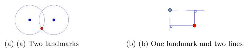
Given two landmarks observations, we may estimate where the robot is as shown in Figure 1a. Note that we end with two hypotheses, which may be chosen at random. In our case, one of them will usually fall outside of the soccer field, thus may be discarded. If more than two landmarks are seen in the current cycle, two landmarks are chosen at random for each particle which is being resetted. In case only one landmark is seen, but two lines as well (when the robot sees only a corner), we estimate it with the distance from the lines to the robot, as in Figure 1b. Moreover, we add gaussian noises to the landmarks' observations before applying this resetting process to better spread the resetted particles.
Finally, the agent's position estimate is determined by a weighted average of the particles positions. For future work, we expect to determine the parameters using experiments or optimization techniques instead of relying on manual tweaking.
Motion Control
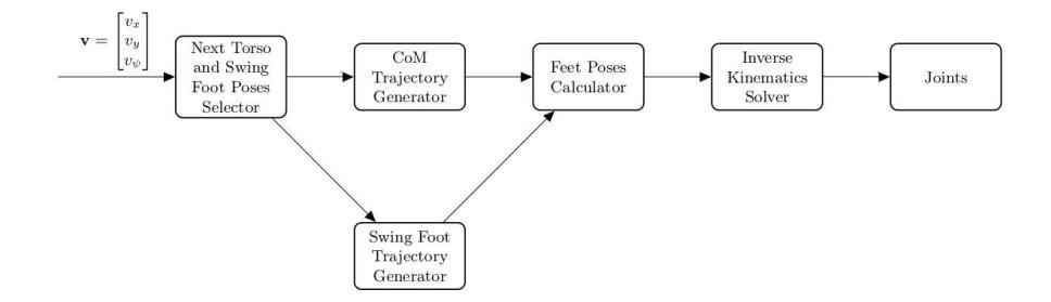
For walking, we use the ZMP-based omnidirectional walking engine described in [9]. In general terms, it follows the flux presented in Fig. 2. The input to the algorithm is the desired velocity v = [vx, vy, vψ] $^{T}$ with respect to the robot's local coordinate system. At the beginning of a new step, poses for the torso and the swing foot are selected for achieving the expected displacement at the end of the step. So, a trajectory for the center of mass (CoM) to follow a reference Zero Moment Point (ZMP) trajectory is computed. The trajectory of the swing foot is obtained by interpolating between the initial and final poses of this foot.
Finally, joints angles are calculated through Inverse Kinematics (IK) considering the poses of the support and swing feet. Note that the module Next Torso and Swing Poses Selector is called once for step, while the others are executed at the update rate of the joints.
Our step planner selects torso and feet poses to make the robot follows an omnidirectional model while respecting self-collision and leg reachability constraints. To reason about the robot dynamics, we approximate it using the 3D Linear Inverted Pendulum Model (3D-LIPM) [1]:
$$\mathbf{x}{ZMP} = \mathbf{x}{CoM} - \frac{z_{CoM}}{g} \ddot{\mathbf{x}}_{CoM}$$
where xZMP = [xZMP , yZMP ] T is the ZMP position, xCoM = [xCoM, yCoM] T is the CoM position, zCoM is the CoM height, and g is the acceleration of gravity. The ZMP is kept at the center of the support foot during single support and moves from the current support foot to the next one during double support. We also use the torso's angular velocities measured by the gyrometer to stabilize the walk.
Dynamic Role Assignment
5.1 Position Model
The Delaunay Triangulation algorithm calculate our player's positions and generate a formation set of agents for every single position of the ball [20]. These positions serve as reference points for an agent to where they should be if there is not any enemy in a dangerous position just according to the ball's position in that moment. The Dynamic Role Assignment [21] idea is that the agents can communicate with themselves, decide the best lineup in that moment and assign the Delaunay Triangulation positions to the team, one for each agent. And do it all dynamically, sending and receiving messages in every communication cycle.
The lineup consists on eleven positions and each agent, using the data received in the World Model, is able to determine which agent should be assigned to each Delaunay Triangulation position based on the agents position. Each position is assigned to a number 1 - 11, just as the agents uniform number. So, the agent generates an array and assigns the number of the Delaunay Triangulation position to each player in its team.
5.2 Communication between Agents
The objective is to send a vector containing each position assigned to each other agent in the team. Each agent can send and receive messages from the server in every cycle of 20 ms, with the messages size limited to 20 bytes (160 bits). The problem is that every integer occupies 4 bytes, and the team has 11 players. So, the vector would have occupy 11*4 = 44 bytes of memory, a lot more than the limit. The solution used was to use the base64 ascii encoder [22], a compression message encoder that creates a bijection between the vector and other structure which occupies less memory. Then, the agents would receive the encoded message and, using the same bijection, be able to decode and receive the message vector. The method proved itself to be very efficient, reducing the size of the role assignment vector form the original 44 bytes to only around 110 - 120 bits.
5.3 Voting System
When the agents have all sent their respective role assignment vectors to each other (they may differ between agent to since their perception is different), they acknowledge the position which was assigned more times to each respective agent. Then, the team's role assignment vector would be filled based on the assignments.
5.4 Marking System
The marking system is a sequential process used to mark opponent agents who are offensively dangerous during the match. The system performs three steps: it decides the players that will be marked, defines roles to mark these players and, finally, uses the Role Assignment system to designate agents for those defined roles. To decide which opponents are to be scored, a heuristic method is used based on the following conditions about the opponent. If it is:
- Close enough to take a shot on goal.
- Not the closest opponent to the ball.
- Not too close to the ball.
- Not too far behind the ball.
After that, a set of formation roles must be selected to mark the chosen opponents. For this, marking roles positions are calculated as the position 1.5 meters from a marked opponent along the line which connects that opponent to the center of our goal. The formation positions to be replaced are the closest to each marking position, and their selection is done by using the Hungarian algorithm, which calculates the minimum sum of distances between the previous forming positions and the marking positions.
Strategy and Decision Making
6.1 Set Plays
As in a soccer game, during a simulated game there are situations where the ball is stopped. When this happens, the team with the ball has a certain amount of time to make a move, while the other team cannot approach more than a certain distance from the ball. For some of these situations we have formulated different set plays, namely: Own Goal Kick, Opponent Goal Kick and Own Corner Kick.
6.2 Robot Navigation and Potential Field
Planning consists of finding a sequence of actions that transforms some initial state into some desired goal state. In our case, we use the Potential Field as our robot navigation method. This technique applies to each field point's point a numerical value that corresponds to the potential caused by external agents. Therefore, is possible to know which points should be avoided and which point is the goal. There are several advantages of using Potential Fields to robot navigation [14]. First, it is easy to implement and visualize, and the resulting behavior of the robot is therefore easy to predict.
Reinforcement Learning Optimization Server
Motivated on the recent advances on Deep Reinforcement Learning, we created a framework that is able to mimic a reference motion and optimize it towards a task. We represented the motion as a neural network, with thousands of parameters, which followed a 2-step training procedure where:
- The first step is a Supervised Learning Training, where we transfer the knowledge from a keyframe representation to a neural network; and
- The second step is a Reinforcement Learning Training, where we optimize the motion from the neural network using rewards related to a specific performance task.
We developed better policies than the initial ones for kick motion. Using this framework, we also showed that pure Reinforcement Learning techniques by themselves will lead to suboptimal policies (due to premature convergence) and will not achieve high performance motions [18].
7.1 Supervised Learning Step
In the first phase, we cloned the kick motion using supervised learning [15].
We acquired the dataset in two different ways. In the first one, we commanded an agent of our team to execute specific motions and sampled the reference joint positions computed by our code. In this case, we sampled the kick and get up keyframe motions [16].
The second approach involved changing the Soccer 3D server source code to provide current joint positions of a given robot, in a similar way as described in [16]. This allowed us to acquire motion datasets from other teams, without any knowledge of how these movements are implemented.
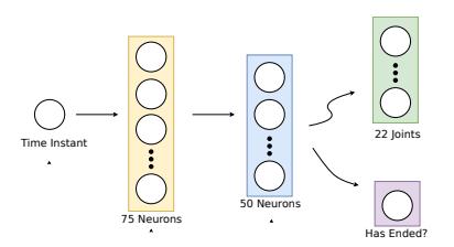
We used a deep neural network with 2 hidden, fully connected layers of 75 and 50 neurons, respectively. The output layer has 23 regression neurons, which represent the 22 joint angles and a neuron which output indicates if the motion has ended or not, as shown in Figure 3.
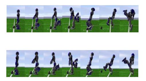
The final mean absolute error was 0.018 radians and the motion was visually indistinguishable from the original one, as can be seen in Figure 4. We performed a test scenario to evaluate the kick motion and compare with the initial policy. Results are summarized in Table 1.
The Kick Comparison
| Kick | Accuracy (%) | Distance (m) Mean | Distance (m) Std |
|---|---|---|---|
| Original Kick | 64.5 | 8.92 | 3.82 |
| Neural Kick | 52.6 | 7.16 | 4.06 |
7.2 Policy Improvement via Proximal Policy Optimization
We optimize the neural network from the Supervised Learning step using the Proximal Policy Optimization algorithm.
Figure 5 shows the architecture used to integrate the learning algorithm, agent and simulation environment. The simulation server exposes a state to the soccer agent, which model this information and passes to the learning algorithm that chooses an action accordingly and returns to the agent. Then, it applies this action in the environment, modifying its state, completing the cycle.
We applied such server in a distributed training setting, using Intel AI DevCloud [19] hardware. We tested the resultant policy and compared with the original and imitated, culminating in the results of Table 2.
As a final experiment, we applied this model to a different kind of robot, the Nao with Toe. When using the original keyframe motion, the Nao with Toe was not able to even kick the ball – very often it kicks the ground because of its large foot. We then applied the framework proposed in this work, which resulted in the values presented in Table 3.
![Reinforcement Learning Server Architecture [17].](/tdps/soccer_simulation_3d__2019__ITAndroids/_page_9_Picture_4.jpeg)
Kick Comparison - Effective Evaluation
| Kick | Mean | Std | Distance X(m) Mean | Distance X(m) Std | Distance Z (m) Mean | Distance Z (m) Std |
|---|---|---|---|---|---|---|
| Original Kick | 9.05 | 3.44 | 0.21 | 0.49 | ||
| Learned Kick | 4.82 | 4.46 | 0.12 | 0.21 | ||
| HLM+RNR Kick | 7.07 | 3.55 | 0.36 | 0.57 | ||
| HLM+RNR+RET Kick | 8.26 | 3.09 | 0.48 | 0.49 |
Kick Evaluation - Nao with Toe
| Kick Type | Accuracy (%) | Distance X(m) Mean | Distance X(m) Std | Distance Z (m) Mean | Distance Z (m) Std |
|---|---|---|---|---|---|
| Nao with Toe | 95.0 | 9.47 | 3.43 | 0.66 | 0.63 |
Conclusion and Future Work
This paper showed the latest developments of ITAndroids Soccer 3D. During Robocup 2018, it was clear that our positioning in the field, In addition to the robot navigation to a desired position were performing below expectations. Now aware of this, we will focus on developing positioning strategies to improve this performance, as well as tools for parameter optimization and machine learning use.
Acknowledgment
We would like to acknowledge the RoboCup community for sharing their developments and ideas. Specially, we would like to acknowledge Magma Offenburg team for sharing their code and, with that base, helping us develop our current code. We thank our sponsors Altium, ITAEx, Metinjo, Micropress, Poliedro, Poupex, Rapid, Solid Works, and Intel. We also acknowledge Mathworks (MAT-LAB), Atlassian (Bitbucket) and JetBrains (CLion) for providing access to high quality software through academic licenses. We would also like to show our gratitude to Patrick MacAlpine from UT Austin Villa team for sharing their ideas and code regarding the Soccer 3D simulation server modification. Special thanks for the cluster access provided by Intel, which raised our computing capacity to a whole new level.
References
- S. Kajita, F. Kanehiro, K. Kaneko, K. Yokoi, and H. Hirukawa. The 3D Linear Inverted Pendulum Mode: A Simple Modeling for a Biped Walking Pattern Generation. In Proceedings of the 2001 IEEE/RSJ International Conference on Intelligent Robots and Systems.
- MacAlpine P., Urieli, D., Barrett, S., Kalyanakrishnan, S., Barrera, F., LopezMobilia, A., tiurc, N., Vu, V., Stone, P.: UT Austin Villa 2011 3D Simulation Team Report. Technical Report, The University of Texas at Austin, Department of Computer Science, AI Laboratory (2011).
- Haider, S., W., M.A., Raza, S., Johnston, B., Abidi, S., Sharif, U., Raza, A. Karachi Koalas3D Simulation Soccer Team, Team Description Paper for RoboCup 2012.
- Dellaert, F., Fox, D., Burgard, W., Thrun, S.: Monte Carlo Localization for Mobile Robots. In: IEEE International Conference on Robotics and Automation (ICRA99).
- Hester, T., Stone, P.: Negative Information and Line Observations for Monte Carlo Localization. In: IEEE International Conference on Robotics and Automation (ICRA08).
- MUZIO, A. F. V. ; AGUIAR, L. G. G. ; MAXIMO, M. R. O. A. ; Pinto, S. C. . Monte Carlo Localization with Field Lines Observations for Simulated Humanoid Robotic Soccer. In: Latin American Robotics Symposium, 2016, Recife. Proceedings of the 2016 Latin American Robotics Symposium (LARS).
- Coltin, B., Veloso, M.M.: Multi-Observation Sensor Resetting Localization with Ambiguous Landmarks. In: Proceedings of AAAI11, the Twenty-Fifth Conference on Artificial Intelligence, San Francisco, CA.
- AGUIAR, L. G. G. ; ALBUQUERQUE, M. R. O. A. ; PINTO, S. C. . Monte Carlo Localization for RoboCup 3D Soccer Simulation League. In: Brazilian Humanoid Robot Workshop (BRAHUR), 2016, So Bernardo do Campo. Monte Carlo Localization for RoboCup 3D Soccer Simulation League.
- MAXIMO, M. R. O. A. Omnidirectional ZMP-Based Walking for a Humanoid Robot. Masters thesis, Aeronautics Institute of Technology, 2015.
- THRUN, S., BURGARD, W., FOX, DR.: Probabilistic Robotics. MIT Press (2005).
- KALMAN, R.E.: A New Approach to Linear Filtering and Prediction Problems. Transactions of the ASMEJournal of Basic Engineering 82, pp. 3545 (1960).
- SMITH, A.F.M., GELFAND, A.E.: Bayesian Statistics Without Tears: A SamplingResampling Perspective. American Statistician 46, pp. 8488 (1992).
- Bruno, Marcelo G.S. Sequential Monte Carlo Methods for Nonlinear Discrete-Time Filtering. Synthesis Lectures on Signal Processing, January 2013, Vol. 6, No. 1, Pages 1-99.
- HELLSTROM, T. Robot Navigation with Potential Fields. Department of Computer Science, Umea University, 2011.
- MELO, L. C., MAXIMO, M. R. O. A, and CUNHA, A. M. Learning Humanoid Robot Motions Through Deep NeuralNetworks.arXiv e-prints, page arXiv:1901.00270, January 2019.
- MACALPINE, P., COLLINS, N., LOPEZ-MOBILIA, A., and STONE, P. Ut austinvilla: Robocup 2012 3D simulation league champion. RoboCup 2012: Robot SoccerWorld Cup XVI, pages 7788, Berlin, Heidelberg, 2013. Springer Berlin Heidelberg.
- MUZZIO, A. F. V. Deep reinforcement learning applied to humanoidrobots, 2017.
- MUZZIO, A. F. V. A Deep Reinforcement Learning Method for Humanoid Kick Motion, 2018.
- Intel AI DevCloud, https://software.intel.com/pt-br/ai-academy/devcloud. Last accessed 15 Jan 2019.
- Pires, F. B.: Regular triangulations and applications (Doctoral dissertation). Retrieved from http://www.teses.usp.br/teses/disponiveis/55/55134/tde-26082008- 163553/pt-br.php.
- Patrick MacAlpine, Francisco Barrera, and Peter Stone. Positioning to Win: A Dynamic Role Assignment and FormationPositioning System. In Xiaoping Chen, Peter Stone, Luis Enrique Sucar, and Tijn Van der Zant, editors, RoboCup-2012: Robot Soccer World Cup XVI, Lecture Notes in Artificial Intelligence, Springer Verlag, Berlin, 2013.
- S. Josefsson. The Base16,Base32,and Base64 Data Encodings. IETF. October 2006. Retrieved from https://tools.ietf.org/html/rfc4648.