ITAndroids Soccer3D Team Description Paper 2023
Arthur Costa Stevenson Mota, Bruno Benjamim Bertucci, Deodato Vasconcelos Bastos Neto, João Lucas Rocha Rolim, Juliano Yoshiro Nishiura, Marcos Ricardo Omena de Albuquerque Máximo, Pedro Pinheiro Borges, Victor Antonio Batista Caus
Autonomous Computational System Laboratory (LAB-SCA), Aeronautics Institute of Technology (ITA), São José dos Campos, São Paulo, Brazil
Abstract ITAndroids is a robotics competition group associated to the Autonomous Computational Systems Laboratory (LAB-SCA) at Aeronautics Institute of Technology (ITA). ITAndroids is a strong team in Latin America. Our 3D Soccer Simulation team started its activities in 2012. Currently, our code is written in C++. This paper guides the reader through the most important features of our code and work tools developed, with a focus on the most recent developments.
Introduction
ITAndroids is a robotics research group at the Aeronautics Institute of Technology. As required by a complete endeavor in robotics, the group is multidisciplinary and contains about 60 students from different undergraduate engineering courses. To motivate our research, we participate in robotics competitions. In the last 11 years, we achieved good results in competitions, especially in Latin America.
This paper describes our development efforts in the last years and points out some improvements we want to implement in the near future. Sec. 2 describes our team's code structure. In Sec. 3, our new kick optimization was described. Sec. 4 explain our model's inference migration to TensorFlow Lite. Sec. 5 presents an implementation of a velocity saturation to avoid agent falls. Sec. 6 we show our optimization to agent's get up using CMA-ES. Sec. 7 concludes and shares our ideas for future work.
Code Structure
The code has been planned and divided into several modularized parts so that each part can be separated from the others with ease. Basically, it is divided into 7 layers. Each of them will be described in this section.
Communication
It is the layer that directly connects with the server, in order to receive messages and send messages through sockets. This layer receives and sends a string as described in the server's website, following the protocol described in the Simspark documentation.
Perception
The Perception layer is responsible for turning the strings received by the Communication layer. This layer parses the string and converts it into a tree. The layer then iterates over the created tree and creates new objects (perceptor objects) from it, so that the agent can have new information each new loop. Each perceptor is as described in Simspark's website.
Modeling
Modeling basically models the world state. It executes probabilistic stochastic filters to determine where the robot is in the field, and where the other agents are. Modeling is divided in two parts, a World Model and an Agent Model.
Agent Model
The Agent Model models information related to the robot itself. It computes transformation matrices which are used to transform vision observations from the camera coordinate system to a coordinate system on the ground.
World Model
The World Model is responsible for modeling world states such as game state, time, and position, so that this information can be used by Decision Making. It runs the Localization algorithm in order to estimate the robot's position.
Decision Making
Decision Making is a layer that gives each agent a role. The roles assigned dictate the movements the agent should take in order to successfully follow a determined strategy. One agent cannot change its role, but, that role must be able to integrate all the possible behaviors the agent has available, e.g. a regular agent receives the AttackingRole, while a goalie receives a GoalieRole. Decision Making is also responsible for calling the Marking System to assign the navigation targets for each agent. After the Behaviors are executed, the action requests generated by them are updated.
Behaviors
Behavior is a set of what the agent can do in order to change its own state. It is a set of instructions that goes from high to low level of abstraction, in order to make the agent follow its strategy.
Each behavior can use other behaviors for a more abstract level of problem solving. For example, Attack behavior can call upon NavigateToPosition so that it does not have to be reimplemented in Attack. Each behavior creates an action request, that is a communication interface with the Control layer, and it is how the agent knows which specific action to take.
The Behavior layer (it is not exactly a layer, since it is part of Decision Maker) has two parts, a part that is a data structure called BehaviorFactory, and a structure called Behavior. A BehaviorFactory stores all behaviors, and each behavior has access to all other behaviors through the Behavior Factory.
Control
Control is the layer that gets the requests from behavior and changes it into more concrete things. For example, it takes a walk request created from one of the behaviors and converts it into joints positions. It is where the movement algorithms are implemented.
Action
The Action layer is responsible for converting all information that the agent has created and that it wants to send to the server to a string in a way that the server can recognize. Then, this string is sent to the server through the Communication layer.
CMA-ES for Kick Optimization
As described in previous TDPs, our team has a kick learned through a neural network. That kick works well in Standard NAO and NAO with toe, but is not the same for Secondary NAO. In order to overcome this problem, we used CMA-ES [1] to find a better adaptation of our kick for Secondary NAO.
The training method used for this kick was quite different from the methods we used previously. In this one, the agent's approach to the ball was considered an attempt to avoid losing the opportunity to kick.
We used CMA-ES to find the best combinations of key frames for agent use. Each key frame was tested several times, and the reward function (1) was computed based on statistical metrics (mean and standard deviation).
$$\text{reward} = \bar{h} - \bar{d}y + \bar{d}x \cdot \frac{3}{4} - f \cdot \frac{4}{5} - \left(\frac{\sigma{d_x}}{3} + \sigma_h + \frac{\sigma{d_y}}{2}\right) \cdot \frac{1}{2}$$
Where $h$ is the height of the ball during the movement, $d^x$ is the distance between the initial and final point on axis x, $d^y$ is the same for axis y and $f$ is the number of falls until the agent could really kick. The numbers multiplying are the parameters' weights. They are adjusted to normalize the maximum value expected of each parameter, the denominator of the fraction, and the numerator according to the importance of that parameter.
We consider that the kick that Secondary NAO agent learned now has a performance similar to the kicks that other types of agents in our team use, both in execution time, and accuracy. We also hope to devise other strategies to create better kicking motions for all types of agents in the near future.
Migration from TensorFlow v1 to Tensorflow Lite
Since 2016, we have used TensorFlow v1 [2] to make the model's inferences, which was the option our team considered optimal at the time. Currently, however, it has been discontinued, and alternatives, such as PyTorch [3], TensorFlow v2 and TensorFlow Lite have shown themselves as reliable substitutes.
TensorFlow Lite is a mobile library for deploying models on mobile, microcontrollers, and other edge devices. Because of that, TensorFlow Lite is lighter, and its inferences are faster than those of other frameworks. Additionally, this tool is easier to integrate and maintain. For the reasons described previously, we opted for TensorFlow Lite.
To make this transition, our team had to adapt all classes with neural networks models, and rework a significant portion of the configuration files used to build the code.
Navigation Helper
Like described in Subsection 2.5, our code has a control layer to translate the movement request into a actual movement. However, the agent cannot walk at all the requested speeds. Because of that, we have saturations of velocities for axes x and y, but there is no saturation given an angle and an angular velocity.
Equations (2), (3), (4) and (5) were previously used to determine the saturation walking speed in a particular direction.
$$\theta_{\text{factor}} = 1 - \min\left[\frac{\omega}{\omega_{\max}}, 1\right]$$
$$v_n = \left(|\hat{v}.x| \cdot v_{\max} + |\hat{v}.y| \cdot v_{y,\max}\right) \cdot \theta_{\text{factor}}$$
$$s = \min\left[v_n, |v|\right]$$
$$v_{\text{walk}} = \hat{v} \cdot s$$
Where $\hat{v}.r$ is the normal vector of $v$ in $r$ direction, $v_{\max}$ is maximum velocity in forward or backward direction. This was not accurate at all, but it worked reasonably well in past years. However, a better method is needed to continue to improve in the league.
To solve this problem with a more efficient method, we use a data-driven solution. We want to find the velocity saturation given $\omega$ and $\theta$, angular velocity and angle. Given those parameters, the agent begins walking with a very low velocity and gradually increases it until the agent falls, which is the saturation velocity; we then save all of this information to train a neural network.
We run the previously described test for $\omega \in [-2\pi, 2\pi]$, our maximum angular velocity, and for $\theta \in [0, \pi]$, assuming the agent's symmetry. A neural network was trained to trace this curve using the information that had been collected. The model was trained with Keras [4] and transformed into a TensorFlow Lite model, in accordance to Sec. 4.
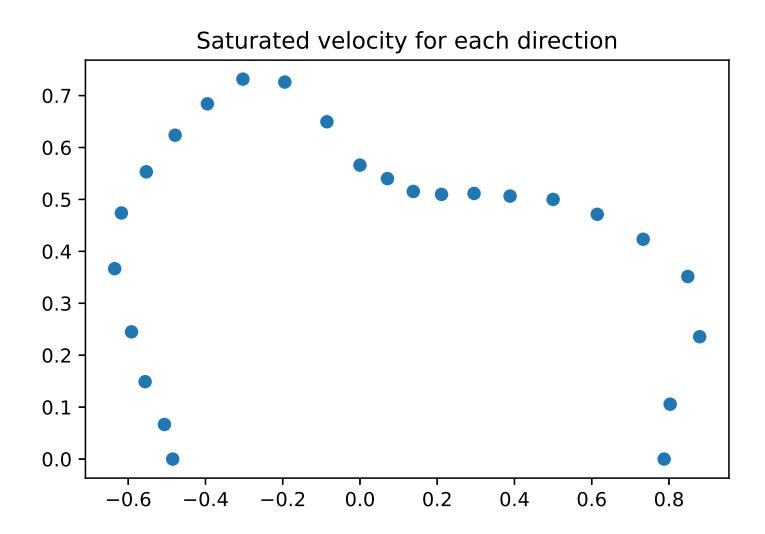
Using a total of 11,265 parameters, the trained model has an input layer with 128 neurons, three hidden layers with 64, 32, and 16 neurons, respectively, and an output layer with one neuron. We chose ADAM as the optimizer and used mean square error as the loss function. Figure 1 is the prediction of the model when the angular velocity is zero and the linear velocity's angle changes from 0 to $\pi$. The result shows a non-linear response, as expected.
CMA-ES for Get Up Optimization
Our agent's old movement to get up was quite unstable, so he frequently falls when attempting that movement. In an attempt to solve this problem, we use CMA-ES to find the best group of key frames to get up. In the optimization, the agent starts lying on the floor, then tries to do the movement to get up. The reward function associated with the optimization was straightforward: the sum of the height of the agent's center of mass at each simulation timestep. This encourages it to get up as quickly as possible, and to stay upright, which ultimately leads to a movement that is fast and reliable.
To evaluate the new set of key frames, a test based on Monte Carlo's technique was used. First, the agent is positioned in the middle of the field and forced to fall. Then, it starts to performing the optimization movement. At the end of the episode, the test records whether the agent's center of mass is above a certain threshold, at which point we conclude it must still be standing, and record the episode as a success. This test was executed a total of 300 times for each key frame, and, while the agent with the new movement, got up in every iteration, the one with the old movement failed in all of them.
Furthermore, that optimization was tested at the most recent Robocup Open Brazil. In that competition, the movement was stable and faster than the previous one.
Conclusion and Future Work
Firstly, we would like to improve our agent's position estimation algorithm, which determine the position of their teammates, the opponents, the ball, and its own. We have determined that the algorithm currently implemented in our agents tends to diverge significantly in situations where it should not.
We are also devising a strategy based on control techniques to improve our agent's behavior when approaching the ball for a kick. The method currently implemented has a very slow convergence, which frequently leads to lost goal, or pass, opportunities.
Also, we are beginning a PID implementation to enhance the movement of the agent's approach to the ball at the moment of the kick. The current method converts quite slowly; this may be due to an imprecise filter or an inaccurate model.
Finally, we will enhance the algorithm for fighting for the ball. Now, based on the states of the agent, such as whether it is standing up, the direction of the player, and other parameters, we utilize a heuristic to calculate virtual distances. We'll approach the issue using a data-driven approach. First, we will run a Monte Carlo simulation to collect data about all possible formations in the field and the best agent to fight for the ball. With that data, we will use an algorithm, possibly an XGBoost, to select the best agent for new situations.
Acknowledgment
We would like to acknowledge the RoboCup community for sharing their developments and ideas. Especially, we would like to acknowledge the Magma Offenburg team for sharing their code and, with that base, helping us develop our current code. We thank our sponsors Altium, CENIC, Intel Software, ITAEx, Metinjo, Micropress, Polimold, Rapid, ST Microeletronics, and Wildlife. We also acknowledge Mathworks (MATLAB), Atlassian (Bitbucket) and JetBrains (CLion) for providing access to high-quality software through academic licenses. We would also like to show our gratitude to Patrick MacAlpine from the UT Austin Villa team for sharing their ideas and code regarding the Soccer 3D simulation server modification. Special thanks for the cluster access provided by Intel, which raised our computing capacity to a whole new level. Altium, CENIC, Intel Software, ITAEx, Metinjo, Micropress, Polimold, Rapid, ST Microeletronics, and Wildlife.
References
- Hansen, N. and Ostermeier, A. (2001) Completely derandomized self-adaptation in evolution strategies. Evolutionary Computation, 9(2), pp. 159-195.
- ABADI, M. et al. TensorFlow: Large-scale machine learning on heterogeneous systems, 2015. Software available from tensorflow.org.
- PASZKE, A. et al., 2019. PyTorch: An Imperative Style, High-Performance Deep Learning Library. In Advances in Neural Information Processing Systems 32. Curran Associates, Inc., pp. 8024–8035. Available at: http://papers.neurips.cc/paper/9015-pytorch-an-imperative-style-high-performance-deep-learning-library.pdf
- CHOLLET, F. et al, 2015. Keras. Available at: https://github.com/fchollet/keras.