B-Smart

Tim Laue, Armin Burchardt, Sebastian Fritsch, Sven Hinz, Kamil Huhn, Teodosiy Kirilov, Alexander Martens, Markus Miezal, Ulfert Nehmiz, Malte Schwarting, Andreas Seekircher

Deutsches Forschungszentrum für Künstliche Intelligenz GmbH, Sichere Kognitive Systeme, Enrique-Schmidt-Str. 5, 28359 Bremen, Germany; Fachbereich 3 - Mathematik / Informatik Universität Bremen, Postfach 330440, 28334 Bremen, Germany

www.b-smart.de

Abstract This Extended Team Description Paper (ETDP) documents the technical state of B-Smart's hard- and software for the season 2009. B-Smart is a project for students in the advanced study period at the Universität Bremen. The team has continuously been participating in RoboCup Small Size League competitions since 2003, including all world championships as well as all major European competitions. This ETDP has been written to fulfill two purposes: To meet the criteria of the SSL Technical Committee, and to help younger teams to have an easier step into the SSL through providing them detailed information about a successfully working team.

1 Introduction

This Extended Team Description Paper (ETDP) documents the technical state of B-Smart's hard- and software for the season 2009.

B-Smart is a project for students in the advanced study period at the Universität Bremen. The team has continuously been participating in RoboCup Small Size League competitions since 2003, including all world championships as well as all major European competitions. The last two consecutive years we advanced to the quarter finals at the world championships where we ended up being beaten both times by Plasma-Z, the later finalist in 2007 and the world champion of 2008.

This ETDP has been written to fulfill two purposes: To meet the criteria of the SSL Technical Committee, and to help younger teams to have an easier step into the SSL through providing them detailed information about a successfully working team. If you have any questions about anything in this ETDP, please do not hesitate to ask us. For further information you can also visit our homepage where you can find former TDPs (among other things).

2 Hardware Architecture

This section describes the hardware architecture of B-Smart's robots.

2.1 Vision Hardware

As almost every team in SSL does, a global vision system is used. For this purpose, B-Smart currently uses two AVT Marlin F046C FireWire cameras which are connected to different buses on a single computer (Pentium IV 3GHz). The cameras are configured to provide the raw Bayer data at a frame rate of about 50Hz.

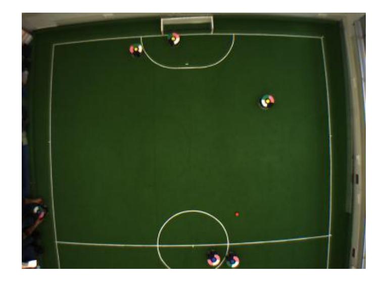
The cameras are equipped with Pentax lenses which have a fixed focal length of 4.8mm. This setup allows us to cover a complete field half (c. f. Fig. 1) even from a suboptimal mounting position. Admittedly, given almost perfect conditions, i.e. mounting the camera exactly above the center of a field half in a height of 4m, a somewhat longer focal length would provide better results.

2.2 Motors

Four Faulhaber 2342S006CR DC-Motors are connected with gear wheels in a ratio of 12 : 1 to actuate the robot. For each motor, a quadrature decoder (LS7366 ) with integrated counters handles the motor's encoder input. Their values can be read through a serial interface. This solution ensures a better resolution for speed measurement without wasting processor cycles of the micro controller.

2.3 Electronic Design and Fabrication

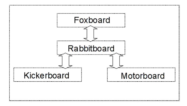
The robot's current electronic design is separated by duty. Each part has its own scope and is therefore swapped into an own PCB (printed circuit board), which leads in our setup to four different components (as depicted in Fig. 2): The Foxboard, the Rabbitboard, the Motorboard, and the Kickerboard. Due to this modular design, it is possible to replace damaged parts easily, which is an advantage especially in the short periods between the matches at the RoboCup. Furthermore, detecting errors on one small component will be faster in most cases than checking one big board which contains all features.

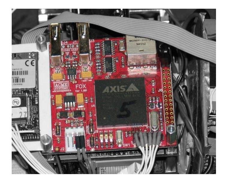
Foxboard High-level control and communication is the main purpose of the Foxboard (c. f. Fig. 3), a MIPS-based embedded board with an Axis ETRAX 100LX 32-bit CPU at 100MHz clock-speed. It offers 40 I/O pins for connecting expansion boards or own devices. A couple of these are used as RS232 serial-ports to communicate with the Rabbitboard and to interface the DECT and Amber Wireless communication modules, offering a wireless link to the PC running the control software.

The Foxboard's operating system is an embedded Linux with kernel version 2.4, which was customized to fit the latency requirements by the simultaneous use of our three communication interfaces.

Rabbitboard The Rabbitboard controls the speed of the four motors with a 200Hz PID control loop. Furthermore, it monitors all important hardware states, especially the light barrier and the battery, and triggers the shooting-mechanism via the Kickerboard. Contrary to the Foxboard, the Rabbitboard was designed by members of the team in 2006 and was improved in 2007. The current version is controlled by an AVR ATmega128 placed on a TQFP (Thin Quad Flat Pack).

The ATmega128 contains an integrated 10-bit-A/D-Converter (Analog to Digital Converter), which is used to determine the remaining voltage of the battery. The ADC selects one channel by using a Multiplexer and compares its value with a reference voltage. The internal reference voltages AVCC are not used for the comparison, instead the VREF with nominally 5V supplies a more accurate comparison.

The Light barrier has a more sophisticated setup. The infrared light emitting diode (IR-LED) quickly changes between on and off in a rate of 88, 06kHz. This pulsed IR-LED has a more powerful light beam than an ordinary one. Since it is known when it is on and off, the misinterpretation of different infrared light can be avoided. For this setup, another IC (ATtiny) has been integrated in the board. Its only purpose is to pulse the IR-LED and to watch how much infrared light reaches the IR-Diode within the same cycle.

The Rabbitboard also manages the shooting-mechanism, which includes disabling or enabling the charge pump of the capacitor and triggering a chip- or a normal kick by setting pins high or low, which are connected to the Kickerboard.

Kickerboard The Kickerboard is directly controlled by the ATmega128 on the Rabbitboard. A charge pump can be activated to charge the 2200µF capacitor to 200V . To charge a capacitor with a power supply of only 12V to a much higher value, the self induction effect of a coil is used: when toggling power supply to a coil, for a short period of time the voltage is much higher than the previously supplied voltage. We use a n-channel MOSFET and an IC (LM3578 ) to constantly toggle the power supply to the coil. the emerging voltage peaks actually charge the capacitor. If the desired voltage has been reached, the charge pump is deactivated.

When the capacitor is charged, two high power MOSFETs can be activated to use the chip kick or the normal kicking-mechanism. The strength of the kick can therefore be varied from 0 to 8m/s by the micro controller, which opens the MOSFET for a certain time (from 64µs to 1ms).

To kick and chip the ball we use two different solenoids. The solenoid for our forward kicking mechanism is 60mm long, has an outer diameter of 35mm and an inner diameter of 13mm. We use a copper wire with ≈ 440 windings. For the chip kick, we are using a pulling solenoid from R+S.

If we send a shoot or chip command to our robot, it first checks, if the light barrier is interrupted. If this is the case, the robot shoots/chips directly, otherwise it will wait for the light barrier becoming interrupted within the next 500ms.

Motorboard The Motorboard is used for driving and monitoring the four attached motors via H-Bridges (VNH2SP30). The maximum current they are able to apply to each motor is 30 Ampere(A), which causes the software to have a certain overload protection. A blocking motor could cause serious damage to itself and other components, therefore the (Rabbitboard's) software monitors the motor's current and prevents further movement of a stuck motor.

2.4 Mechanical Design and Fabrication

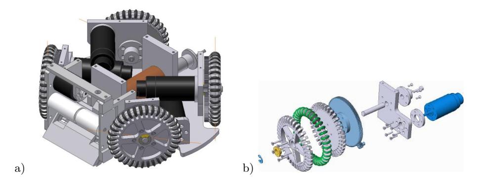
The main chassis consists of two laser-cut aluminum plates which are connected by four motor mounts. The robots have a diameter of 177mm, their height is 144mm. The driving system consists of four wheels (c. f. Fig. 4a) having 36 subwheels each (c. f. Fig. 4b). The back wheels have an angle of 45◦ to the roll axis and the front wheels 53◦ .

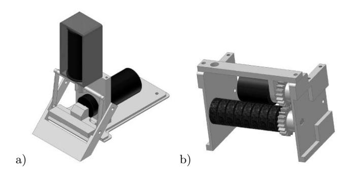
The robot has a low shot kicking mechanism for straight and hard shots and low power passes. There is also a chip kick for high passes (c. f. Fig. 5a). Above the kicking mechanism, a dribbler is mounted (c. f. Fig. 5b), which is driven by a Faulhaber 2224U006SR DC-Motor and connected to the axis of the dribbler by an o-ring. To comply with SSL rules, the dribbling system and the chassis conceal only 18 percent of the ball.

2.5 Batteries

Each robot is equipped with one Graupner LIPo 3/2000 G2,7640.3 lithiumpolymer rechargeable battery, with a capacity of 2000 mAh and 11.1V per cell.

In a typical RoboCup match, a fully charged battery lasts at least one half (10 minutes). Depending on the role the robot is playing, e.g. the goalie, it might not be necessary to change the battery during the game at all.

3 Software Architecture

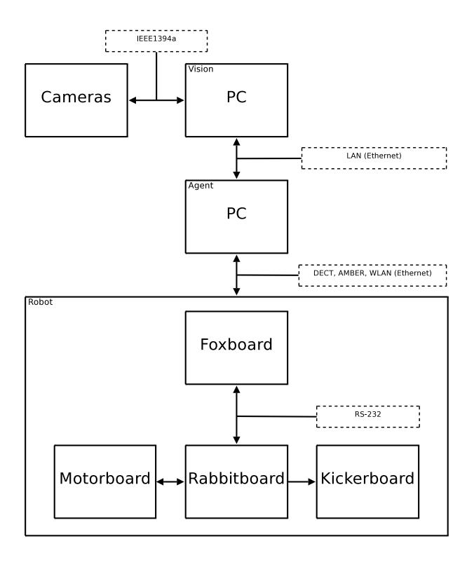
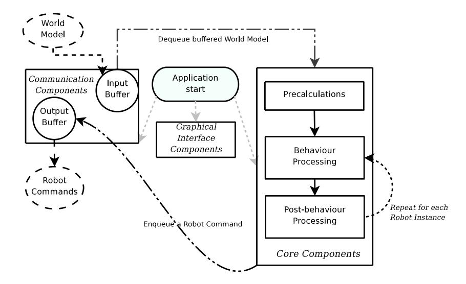
The main part of our software system is composed of a sequence of applications (c. f. Fig. 6). First, we have the Vision, which is responsible for image reception and object detection (described in Sect. 3.2). It transmits the calculated world model to the Agent. This application computes the behavior of each agent (virtual robot instance) and the corresponding motion vectors (c. f. Sect. 3.3, Sect. 3.5, and Sect. 3.4). The next component is the software running on the embedded Foxboard in each robot. It receives the appropriate motion vectors through our communication stack (c. f. Sect. 3.7) and transmits them to the Rabbitboard micro controller, which executes necessary PID calculations and actuation.

The secondary part contains some auxiliary tools we use to aid debugging and behavior development. We have a Logplayer, which records and replays world models and allows us to replay game logs without the need of the computing power of a vision system. We also have a simulation application which is based on the ODE physics engine and OpenGL (c. f. Sect. 3.8).

3.1 Software Environment

Most parts of our software are written in standard C++ with STL. The programs that run on the robot's hardware are written in C (standard and for AVR micro controller). We currently use Ubuntu Linux as default operating system. This provides the team members a common development platform. Our software utilizes many external open-source libraries. Here is a short overview of most of these libraries and what we use them for:

libdc1394 http://damien.douxchamps.net/ieee1394/libdc1394 This is a library for communicating with IEEE1394 digital cameras. We use it in our Vision to setup camera properties and to acquire images.

opencv http://sourceforge.net/projects/opencvlibrary A popular computer vision library. We use it only for camera transformation calculations.

fftw3 http://www.fftw.org A popular library for computing discrete Fourier transforms. The name comes from "Fastest Fourier Transform in the West". It is used by our HSV segmentation module.

gsl http://www.gnu.org/software/gsl This is the GNU Scientific Library. We use it mainly for robot noise in our simulator.

gtkmm http://www.gtkmm.org This is the official C++ interface of GTK+. We use it's libraries (gtkmm, glibmm, glademm) extensively in our user interfaces.

libsigc++ http://libsigc.sourceforge.net This library provides a type safe C++ callback and signaling API. Besides by the GUI it is also used by our network controller. The XABSL (3.4) library also requires and uses this library.

sdl http://www.libsdl.org The Simple DirectMedia Layer provides a cross-platform interface to media devices. We use it to display our world model and to debug information graphically. It is also used by our simulator.

ode http://www.ode.org The Open Dynamics Engine is a popular library for rigid body simulations, providing the base for our simulation application.

OpenGL http://www.opengl.org We currently use it only for 3D visualization in our simulator.

3.2 Vision Software

The Vision computes the world model for the agent. For this purpose, it grabs the images from the cameras, extracts the needed information, and generates the abstract representation of the world, which is then transmitted to the agent.

In order to aid debugging, the application is divided into two basic module groups: Image Processor and Post Processor. Each camera has its own Image Processor, which extracts the information from the camera image. Afterwards, the Post Processor integrates the information from both image processors to one world model. Additionally, the world model is expanded by some external information (e.g. the gamestate from the referee box, and feedback sent by the robots).

Image Processor The Image Processor is a stack of modules which have the task to determine the position of all relevant objects on one field half. To complete this task, all of these modules have access to the image, an additional data structure for temporary (and maybe by other modules needed) calculation results and a data structure which will finally be passed to the Post Processor.

The first goal is to reduce the amount of data to a minimum. Therefore, our system contains a ROI Detection (region of interest) module. The basic idea is to recognize areas in the camera picture where the robots or the ball could be. The combination of three methods (information about previously detected blobs, difference of two pictures, and detection of contrast regions) provides a stable identification of regions where possible objects can be recognized later. This process reduces the amount of false blob detections and minimizes data needed for follow-up calculations. In addition, a Masking module sets all definitely unneeded pixels (i.e. the area not belonging to the field) in the image to black.

We use a HSV-based color segmentation approach for detecting the colors of robot markers and the ball. The HSV color model provides a more stable color classification when used in environments with changing luminosity (e.g. dynamic highlights and shadows on the field). This is due to the fact that the hue component of the physical object color stays relatively constant when the light intensity falling on it changes. To perform color segmentation, a Fast Fourier Transformation of the picture is used to set thresholds in each color class and to build a look-up table used later for real-time color classification.

The RLE Compression module segments the three important colors (blue, yellow and orange) and compresses these information by Run Length Encoding. During this compression process, multiple pixels with the same color are grouped to one pixel with the additional information how often this color appears. After the compression the image is represented by a lists of such runs.

Based on this representation, the Blob Detector module now determines by means of configurable values (e.g. minimum/maximum size, momentum) all significant blobs within the RLE image.

The blobs allow an easy Ball Detection as well as a basic Opponent Detection which does not take the orientation of the opponent robots into account.

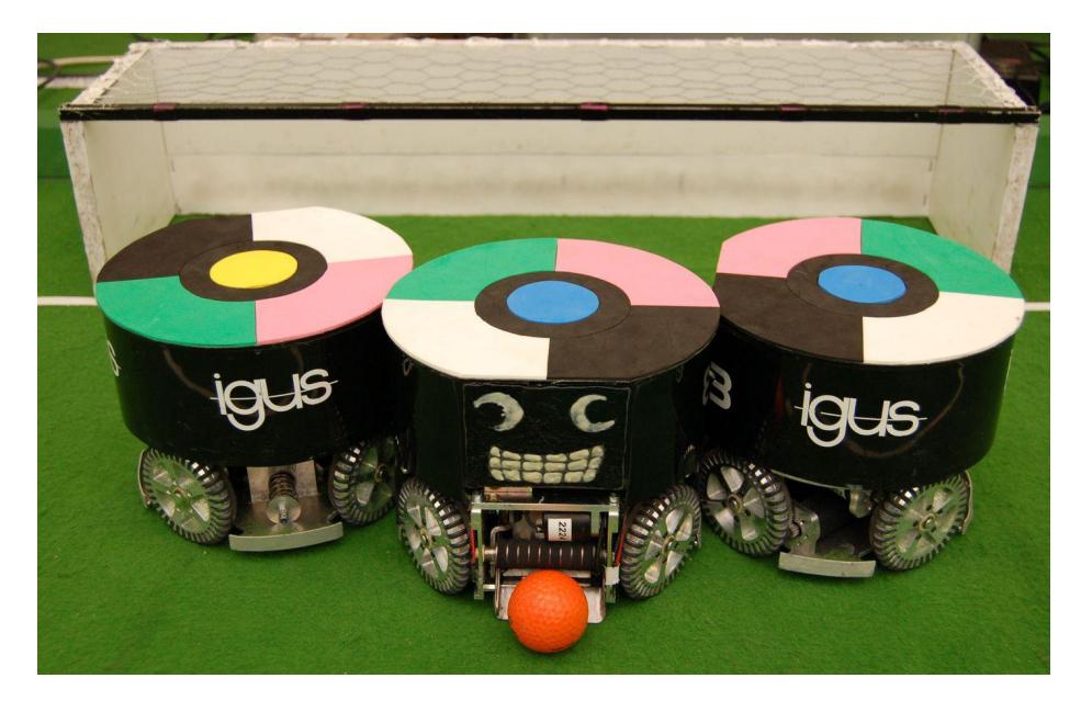
To detect the detailed information about the own robots, i.e. the identity and the rotation, the center blob is used as starting point for some further image processing performed by the Team Detection module. Our circular cover (c. f. Fig. 7) consists of four colored (and simply distinguishable) areas of the same size. The order of the colors (black, white, magenta, green) encodes the ID, whereas the black field is always located left of the front to indicate the robot's orientation. This information is extracted by directly comparing the color values of the pixels around the center blob. This can be done without any previous color calibration. Furthermore, to ensure a reliable detection of the marker's center, a black ring separates the four fields from the center blob.

Post Processor The Post Processor modules receive a data structure from each Image Processor which contains the computed position of each object in our field coordinate system.

The most important basic operations of the Post Processor stack are to merge the information from both perspectives – as an object could be in both camera images – and to control the adding or removing of objects to the world model sent to the agent. The latter is important to filter out false positives as well as to bridge short periods of time in which an object was not seen.

For organizational reasons, some minor tasks are also executed: The Gamestate module receives information from the referee box and attaches them to the world model. For testing purposes, it is also able to emulate a local referee box. The Robot Feedback module adds the feedback from the robots (e.g. the light barrier state) to the world model.

In addition to the more or less organizational tasks fulfilled by these modules, the Post Processor also has to smooth the noisy, unfiltered perceptions computed by the Image Processors. In previous years, the velocities of the ball and the robots were measured by plain differences of positions in a certain time. This is sufficient to gain a rough estimate but leads to problems when algorithms like path finding or behavior routines depend on this value. Reasons for this inaccuracy can be found in the noise of the compressed image data with small resolution and changing lighting conditions. Moreover, these effects are amplified by slight miscalculations or improper software configurations. Changes of only a few pixels in position can cause big noise on the velocity value.

To reduce the effects mentioned above, a compensation algorithm was implemented. The idea was to feed one filter for each object to track with continuous position data. Based on those measurements and precise time stamps on each picture, the algorithm is able to estimate the position of the moving object. Of central importance for this algorithm are the multiple instances of the objects which are tracked over time. Each one is initialized with the measured position and added random Gaussian noise to simulate the uncertainty of the camera measurement. After this, a velocity vector is determined by pure random noise. Now the second measurement is awaited and every virtual state gets moved as if his position and velocity were true for the passed amount of time. The resulting state is now compared with the real measured one and rated accordingly.

Some cycles later, the virtual states by this converge towards the real state and smooth its changes as one outlier is not able to invalidate the whole set of virtual states. Nevertheless, this convergence also tends to result in problems with high dynamic environments where spontaneous changes in the estimated value, velocity in this case, are likely to happen. Unfortunately, exactly this is what happens if a small size robot just stops in a few milliseconds due to strong motors. To solve this, approaches such as particle injection are utilised. Thereby, in every step some particles are generated from direct camera measurement or hypothetical engine stops. This grants the filter the ability to react faster on sudden changes while estimating not too many states and to keep good performance.

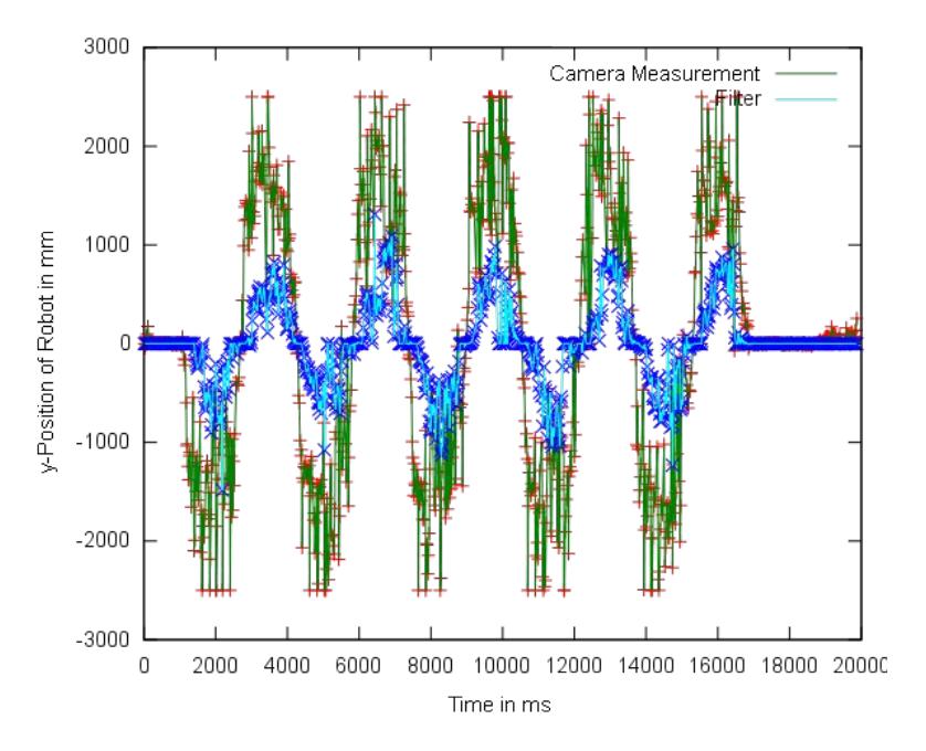
The analysis of the implemented filter revealed that there is a high potential for smoothing the ugly measurements used until now (c. f. Fig. 8). However there are certain drawbacks which might get solved by further refinement of the implementation. This involves e.g. a delayed estimation of up to two frames produced by the converging principle of this method. It might be possible to overcome this by adding additional measurements of motor data and artificially increase the amount of passed time during the estimation of new states. Furthermore, the filter needs many parameters e.g. for noise values or certain thresholds. Resulting from this, the overall filter performance may vary heavily.

3.3 Agent

The Agent provides the artificial intelligence part of the software system. It receives an abstract representation of the world (world model) and calculates motion vectors for each robot of the own team. In order to aid debugging, the application is divided into three basic module groups: pre-behavior, behavior and post-behavior.

The pre-behavior modules extract general but necessary information from the world model, e.g. a proper formation. Some modules try to guess if a previously chosen behavior worked out well for the own team and calculate other data used later in the decision-making.

The behavior modules compute the desired move for each robot. Currently, the main module used is XABSL, which is described shortly in Sect. 3.4. Two small modules which provide additional strategic information to XABSL can be found in Sect. 3.4.

Each robot has its own set of post-behavior modules. Their task is to calculate the motion vector for the previously set destination position. For this purpose, a path planner does the collision detection and obstacle avoidance to find a safe way to the robots' destination (c. f. Sect. 3.5). Afterwards, a PID controller smooths the path. The final control command is then passed to the communication module.

The detailed data flow within the application is depicted in Fig. 9.

3.4 Behavior Control

XABSL The Extensible Agent Behavior Specification Language (XABSL) [1] is an XML-based behavior description language which can be used to describe behaviors of autonomous agents. It simplifies the process of specifying complex behaviors and supports the design of both very reactive and long term oriented behaviors. It uses hierarchies of behavior modules that contain state machines for decision making. XABSL has already been successfully applied by a number of different RoboCup teams, e.g. the GermanTeam [2] in the Standard Platform League.

Behaviors are specified in a C-like programming language and transformed to an intermediate code which is interpreted by the XABSL engine. This shortens the system's compile time, allows more effective behavior development, and becomes very handy when changes have to be applied in the halftime of a running game.

Roles and Positioning The decision which role a robot shall play is made very early in the XABSL-tree. The facts which influence the decision how the team-wide segmentation is done are global facts such as position of the ball, possession of the ball, opponents' positions and manually added properties as the current default formation. The decision which robot gets which role is based on each robot's position towards the ball, towards the opponents and towards the teammates. Additionally, manually set roles (such as the goalie) are considered.

There are currently three different main roles in our behavior. The goalie is a fixed robot which can only be interchanged with the referee's allowance. Our standard formation usually leads to two defenders and two strikers. The robots can interchange between these positions depending on which selection provides shortest distances for getting all positions covered.

Every robot chooses its positioning behavior depending on the assigned role. While striker and defender act similarly when in possession of the ball, they have different tasks when they are not. We differ into four situations:

1. goalie
2. defender
3. striker without ball
4. striker with ball

Goalie The goalie behavior divides into three possible sub-behaviors:

1. clear ball
2. shorten angle without defenders
3. shorten angle with defenders

Whenever the ball is at close range of the goalie, it will try to get the ball out of the dangerous area as fast as possible. If a pass to a teammate is possible and the goalie has enough time to adjust itself, it will take this pass. The receiver should have a certain distance to the own defense area, though, so clearing the ball has priority over bringing the ball back to game.

The most oft executed behavior for the goalie is the play without ball. For this, we calculate the middle of the angle the ball could be shot to score given a goal without any goalie. The goalie will always try to minimize this angle, or as we say: shorten the angle. It will always take the current ball position as orientation point and will not speculate about where the ball could be passed to as this possible situation is already handled by defending teammate covering opponent robots.

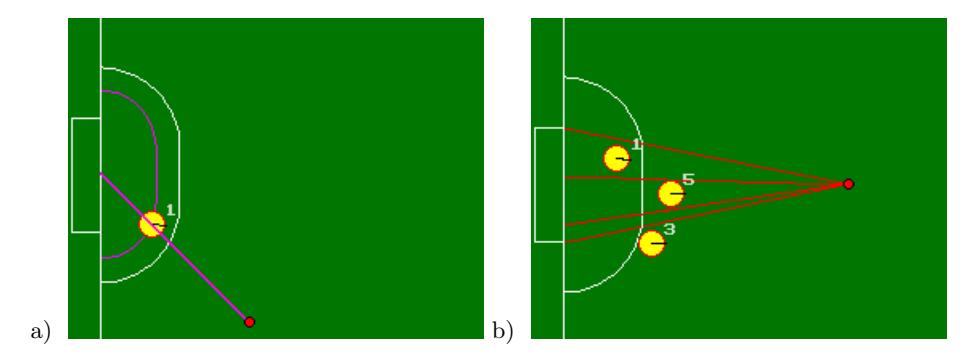
If there are no defenders in front of the own defense area, the goalie positions between the ball and the middle of the own goal. As shown in Fig. 10a, the exact position lies slightly behind the border of the defense area, as in that position the goalie achieves the best result but is still under special protection by law 12.

If there are defenders supporting the goalie in front of the own defense area, especially those in our default defense formation (c. f. Fig. 12), the goalie will try to shorten the remaining angle and to divide it into two similar small ones. If the defender(s) leave two or more angles open for the ball, the goalie chooses the biggest one (c. f. Fig. 10b).

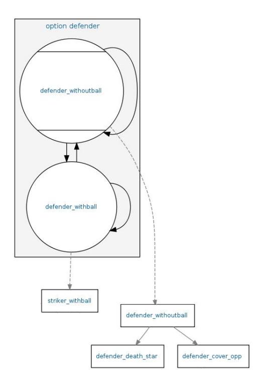
Defender For the defender behavior, it is differentiated whether the defender is in possession of the ball or not. If the defender is at the ball, it will behave like a striker, this can be passing the ball towards another striker, shooting at the goal or dribbling forward.

If not in ball possession, there are three different sub-behaviors. Their selection is chosen depending on a specific weighting. If all robots are available on the field, the selection is as follows:

1. interfere opponent robot possessing the ball (1 robot)
2. join standard defense formation, aka DeathStar (1-3 robots, if available)
3. cover opponent player without ball (remaining robots)

Figure 11 depicts the decisions and interconnections within the defense behavior.

Depending on the manual settings, there can be up to three robots in the defense formation. If there are less than five robots available, the robots will not take tasks with low priority from the list above.

The highest priority is to interfere the opponent ballplayer. For this reason, the robot which is nearest to the ball is chosen to drive towards the opponent robot possessing the ball. The main idea here is to cover the line between the ball and the own goal. To perform this task as fast as possible, even a striker can take this position. Doing so, the defender will try to cover the own goal with highest priority, while the striker will have its priority to get the ball. After all other defenders are in position, the defender attacking the ball may change its objective.

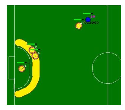
The defense formation is positioned around the own defense area, as shown in Fig. 12. During the game, almost all the time at least one robot is in this position, even if the own team is in possession of the ball. The robot is always covering the line between the ball and the nearest goalpost. The main issue is to support the goalie to defend unexpected shots on the goal. By assigning more than one robot to this position, it is possible to further reduce the angle an opponent robot might hit to score. Primarily in matches against very strong opponents, which are quick and accurate, this is one of the most important tasks to be done.

If one or more robots are supposed to cover opponents, they try to take a position on the line between the own goal and the opponent they want to cover. If the opponent is waiting for a pass in our half, the defender will stay close to him to shorten the angle for a possible shot on goal. If the opponent is waiting for a pass in his own half, the man marker will cover the line in a very defense way. In this case, the defender is staying approximately on the half of the own field side. The motivation of this distinction is to minimize the risk of covering a defensive opponent which is probably able to make a shot on goal, as this position allows to switch quickly to another opponent to cover. Figure 13 shows a possible scenario in a typical RoboCup Small Size League match. The yellow circle shows an opponent (blue team) against his man marker, which is covering the goal shot line. The red arrow points at a defensive opponent that is able to make a dangerous shot on goal. In this case, the man marker stays in his own half and keeps distance.

Additionally it needs to be considered that the man maker is not allowed to drive into the own penalty area. If it would prevent a shot on goal by entering the own defense area, it would result in a penalty for the opponent team. To avoid such a behavior, the man marker switches to a position on the line between the ball and the opponent robot it wants to cover to try to interrupt a possible pass. It will stay in this position as long as the distance between his opponent and the middle mark of the goal is less than one meter.

Criteria for covering opponents Like in real soccer matches, the man marker has to guard opponents that seem to be in a dangerous position. Hence, it is very important to determine which player is supposed to be dangerous. If there are more opponents in dangerous positions than man markers available, a decision has to be made which opponent to cover. This determination is made by several criteria:

• Is the opponent in the opponent part of the field?
• Does it have a good position to make a shot on goal?
• Might it have an easy shot (are there no defenders on the line between the robot and the goal)?
• Might it receive the ball without usage of a chip kick?

Every possible opponent is rated and the robots with the highest value will be covered as long as they are the robots in the most dangerous positions.

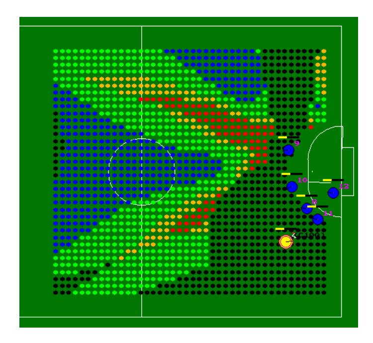
Striker without Ball The striker without ball has a prioritized list of actions to choose from. If the ball is not already moving towards the robot, the striker tries to get to a free point preferring a position that has free lines between itself towards the goal and the ball. To find the best position on the field, a grid of positions of which every single one is rated based on a set of parameters is used (c. f. Fig. 14). As it turned out to be very expensive to recalculate all positions in every cycle, a two-staged system was implemented: First, a wide grid is calculated from which a well rated area of positions is taken, then the positions in the chosen area are rated more precisely. If no position matching the criteria can be found, the striker positions diagonally behind the robot possessing the ball. This leads to a dramatically decreased number of turnovers in duels.

Striker with Ball If the striker is in possession of the ball, there are also several prioritized actions available. Whenever possible, the robot attempts to perform a direct shot on goal through a gap in the opponent line of defense. Even if the gap is closed at once, the striker will stick to this decision for some time to avoid state fluctuation. The gap between the opponent robots must have a minimum width for the striker to consider a shot on goal.

Alternatively, the striker can use a position rating function – similar to the one described in the previous subsection – to find a teammate that is more likely to score a goal and pass the ball to this robot. Otherwise, if no robot matches the minimum requirements, a chip kick pass is taken into account using similar criteria.

If none of these options seem to be profitable the striker tries to play the ball somewhere in the direction of one of its teammates or as a last try, the ball is just shot or chipped towards the opponent goal, no matter if there are opponents in the way.

Dribbling The decision whether the robot tries to dribble or not is very simple. As we use dribbling only as help to keep the ball close to the robot, every robot will start to dribble whenever it is in possession of the ball. There is are no special behaviors for passing the ball in a curve or passing it backwards.

Motion Whenever one of the robots tries to get to a certain position, there are constraints left which the robot must not hurt. For example, the robot may not cross a friendly robot's shooting line if this robot tries to score. When returning to the own defense area, the robot will first try to cover the opponent's shooting line towards the own goal in order to prevent fast scoring by the opponent.

There are also tactical thoughts how to get to the ball. If the own robot is trying to get to the ball and recognizes that an opponent will be there first, it will get between the ball and the own goal first to interrupt the opponent's play as a start. Only after having accomplished that, it will continue attacking the ball.

Interception In a soccer game, it is an important task to intercept a rolling ball. The robot should control the ball as early as possible.

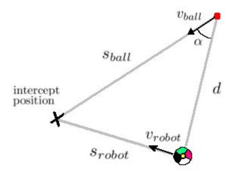
The B-Smart Agent estimates an intercept position that is used as a target position by a robot for interception. This position should be the nearest position in the ball's way the robot can reach before the ball. Given the position, speed, and deceleration of the ball as well as the position, speed, and maximum acceleration of the robot, a good position for interception can be retrieved.

By using equations for uniformly accelerated linear motion the movements of the ball and robot (c. f. Fig. 15) can be calculated with

$$s_{ball} = v_{ball} \Delta t + \frac{1}{2} a_{ball} (\Delta t)^2$$

$$s_{robot} = v_{robot} \Delta t + \frac{1}{2} a_{robot} (\Delta t)^2$$

Given the ball direction and the ball and robot positions, the angle α is known. The equations can be combined with the cosine rule to

$$s_{robot}^2 = s_{ball}^2 + d^2 - 2s_{ball}d\cos\alpha$$

By solving the equation, the time t can be calculated. The intercept position can be retrieved by inserting t in the respective equation.

In the robot equation, the robot is considered to drive towards the intercept position with a constantly increasing speed. This assumption is correct for short distances to the ball. If the robot reaches its maximum speed, the result is wrong, but by recalculating the position in every cycle, the result is improved when the robot gets near the ball.

Strategies The global strategy is to score more goals than the opponent. In addition to the behaviors determined by XABSL, two modules exist to influence and to optimize the decisions leading to our aim. These modules provide the only strategy that does not emerge out of the normal XABSL-decisions.

The Coach is trying to select the best behavior suitable against the current opponent team. For every offensive standard situation, more than one tactical behavior is prepared, which the robots are able to perform. The Coach rates the previously executed behaviors and chooses the best rated. The results are improving, the more situations the Coach evaluates.

The Coordinator system is called after all XABSL-decisions have been made for all robots. It can overwrite and/or redistribute the calculated output symbols, if it detects a possible improvement resulting from the advantage of knowing which decisions have been made for every single robot. The Coordinator also replaces some parts of the XABSL behavior for some behaviors that benefit from a centrally managed control.

3.5 Path-Planning

The path-planning system is based on the "Real-Time Randomized Path Planning for Robot Navigation" approach by Bruce and Veloso [3]. This approach has been used several years by the CMDragons team. The system is a combination of path-planning with Rapidly-Exploring Random Trees (RRT) and a reactive system for collision avoidance, called Dynamic Safety Search (DSS) [4].

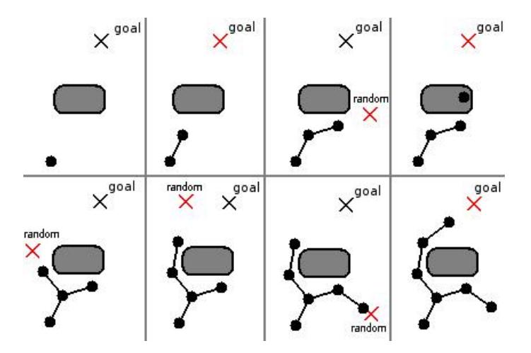
Rapidly-Exploring Random Trees The path-planning system has to find a free path from a given start position to a goal position. In every cycle, the RRT algorithm builds a tree in the state space beginning with a node at the start position. The basic RRT algorithm iteratively executes the following steps, until the goal position is reached:

• Choose a target position for the current iteration. For a given probability p, this target position is the goal position. In the other case, a random position is chosen.
• Get the node of the tree with the lowest distance to the target position. The tree has to be extended at this position.
• Create a new node by going a constant step length from the formerly chosen node towards the target position. To avoid collisions, the new node is added to the tree, if it is not inside an obstacle.

The tree is extended by adding new nodes towards different target positions. Only with a small probability the tree is extended directly towards the goal position. Mostly the target position is a randomly chosen position on the field. Thus it is possible to find a free path around obstacles. Figure 16 shows an example of building the tree.

In [3], this algorithm has been extended by a way point cache (Execution Extended RRT). Once a free path has been found, the nodes on this path are saved as way points. These way points can be chosen in the next cycle as target positions. Because of the short cycle time, most parts of a previously found path can be reused to increase the planning efficiency. This algorithm does not search for the optimal solution. Due to the highly dynamic environment, it is preferable to find some free path within a short time than searching a long time to find the best path.

The state space used for the RRT consists only of two-dimensional field positions. Robot dynamics like speed or acceleration constraints are disregarded. This would lead to a much larger state space and the path planning would not be fast enough. This means that its not always possible to follow a path given by the RRT with maximum speed. Nevertheless, the desired acceleration is set to the maximum acceleration in the direction given by the path. After these accelerations are calculated for all robots, the second part of the path-planning system is used to avoid collisions.

Dynamic Safety Search The result of the path-planning is only a direction for every robot. To drive as fast as possible, the maximum acceleration in this direction is chosen. However, these accelerations are often unsafe, because the robot would not drive exactly along the path. So a reactive system is used to avoid collisions.

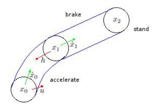
The desired accelerations are checked by the Dynamic Safety Search described in [4]. For every robot, a trajectory is calculated. In the first segment of the trajectory, the given acceleration is executed for one cycle. After this, the second segment executes the maximum deceleration to stop the robot (c. f. Fig. 17). The DSS checks these trajectories for collisions. If an acceleration is unsafe, some other random accelerations are checked. The desired acceleration is overwritten by the most similar acceleration that is safe. If no safe acceleration can be found, it is at least possible to stop the robot without collisions, because this has been checked for the acceleration chosen in the last cycle.

3.6 Motion Control

If the robot has to drive around obstacles to reach its target position, the path planning module is used to create a path and the dynamic safety search gives an acceleration vector. This acceleration is used to create a speed vector for the robot and the PID controlling module is only used for rotation.

If there are no obstacles between the robot and its target position, the PID controlling module computes a speed vector to drive there and stop. The result of this module is a vector with speeds for the x-axis, y-axis, and for rotation. This speeds are calculated using the current robot position, the target position and a position to look at.

Finally, the speed vector for the robot is normalized to a maximum speed, rotated to the robots coordinate system and sent to the robot.

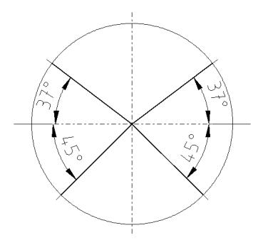
When the robot gets a speed vector, the embedded software converts the desired x, y and rotation speed r of the robot to rotations per minute for each wheel. The conversion is done for an omnidirectional robot (Fig. 18).

Each wheel motor has an encoder chip to monitor the wheel movement. We get 20480 ticks on a full wheel turn. So we can monitor a wheel movement of 0, 02◦ . The wheel speeds are converted to motor ticks per 5ms and a PI control loop at 200Hz generates a PWM Signal.

3.7 Communication Control

This section describes the communication components of the B-Smart team.

Setup We have two separate communication scopes:

1. Wired communication (LAN) among PCs
2. Wireless communication with the robots

The wired communication uses UDP datagrams over Ethernet. Since the Vision and the Agent run on different computers, the most important datagram is the world model from the vision server. The world model from the simulator and robot commands are sent through the cable, too. By using multicast groups, we can work in the same physical net without influencing each other. As all datagrams flow through the Ethernet, it is also easy to record log files.

The wireless communication is only for communicating with the robots. Currently we can use WLAN, Amber Wireless and DECT simultaneously. The drive commands are sent via broadcast to the robots, the robots themselves can send back status information via unicast to the Agent.

Modular implementation As we have a superclass for every communication module, it is easy to implement new medias. To implement a new media it is just required to implement an initialization method, a method to send raw data and a method to receive data.

Sending - The communication kernel holds a list of all available communication modules and the relation robots: robot_id → (media, address), where robot id 0 is reserved for the broadcast address. To communicate with the robots, a program must have an instance of the communication kernel. When sending a packet to a certain robot, the communication kernel searches the subset of robots for the corresponding robot id. For every element in the subset, the data is passed to the communication module that handles the given media using the given address.

Receiving - Once a module has read a packet, it invokes the static process packet function of the communication kernel. This function holds a list of function pointers. If an entry for the current packet type exists, the corresponding function is invoked with the data contained in the packet. Programs can register their functions in their instance of the communication kernel.

Simultaneous usage Since we have different communication media and we discovered that the quality of a medium depends on the environment, we decided to make all media work simultaneously. Additionally, the robots should be able to choose the best medium for communication and they should be able to recognize old packages and drop them. For that reason, we added a TCP like sequence number to our communication protocol.

Sequence numbers As sequence number we use the factor ring Z60000/Z and additionally a special number 61000 for synchronization. Due to the frame time of 20 ms, the sequence number cycles every 20 minutes.

In the communication process, the robot acts as slave, so it has to determine valid packets from the communication stream. When a sending program is started, it uses the special sequence number 61000, which is always valid, for the first 10 packets. After synchronization, a sequence number is valid if it is inside of a certain range starting from the last as valid identified sequence number.

Hardware The communication on the robot is completely handled by the Foxboard. For WLAN, we have attached a WLAN USB stick, the D-Link DWL-122. Additionally, we have serial interfaces on the board to implement serial protocols, in our case DECT and Amber Wireless. The Amber Wireless module is the AMB8420 transceiver module, for DECT we use the Höft & Wessel HW86012 module.

Comparison We discovered that DECT works best in tournament, maybe because of the rarely used frequency band of 1.9 GHz. WLAN also works fine in our laboratory but during a competition, it is the worst medium since a lot of people and other leagues use WLAN, too.

3.8 Simulator

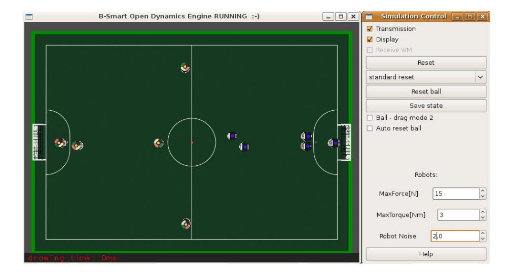
The B-Smart Simulator is a tool to provide the possibility of offline-development and a safe environment for testing high level control code. It receives robot commands sent by the Agent and sends back world models after calculating the changes in robot positioning and ball behavior.

The generated world model is visualized using OpenGL to support the developer with visual feedback (c. f. Fig. 19). To provide the possibility to enforce certain situations for testing, it is possible to interactively change the world state by moving objects.

The Simulator uses the ODE library for rigid body physics simulation. Although the simulation does not reflect the real physics it gives a first feedback to the programmer without the danger of damaging the robots through wrong code and without the need for the programmer to be at the playground.

Since a three-dimensional world state is updated by ODE, the display also uses three dimensions, although a two-dimensional drawing would be sufficient (as in other modules of the B-Smart software).

3.9 Logplayer

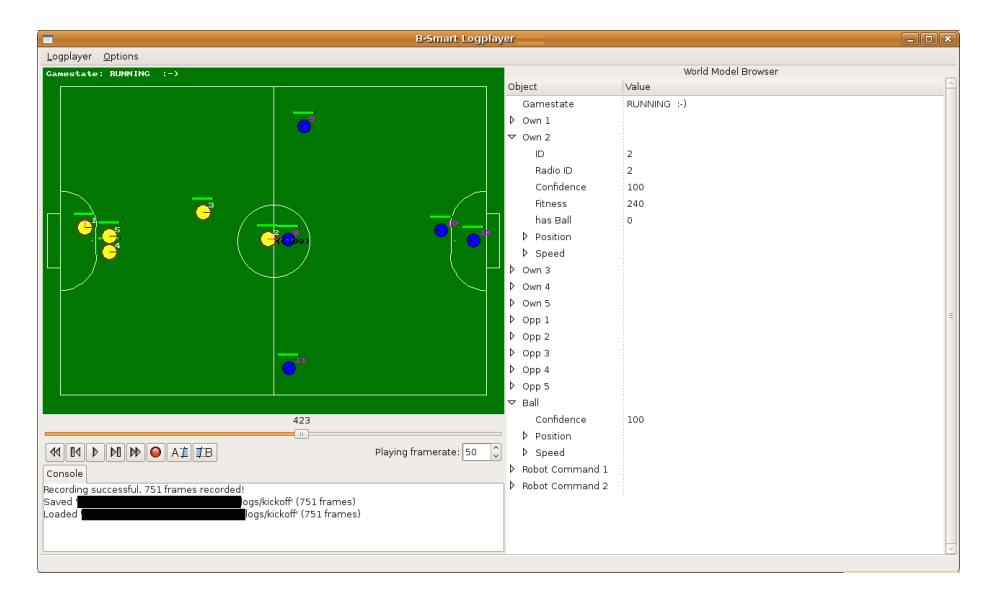
The B-Smart Logplayer is a tool to provide the possibility of recording and replaying games and testings. All world models are written into a logfile which can be saved, loaded, paused, spooled, and viewed frame by frame. In addition to this, every world model is enriched with information by the agent to provide better debugging. All world models and additional information can be viewed in detail in every frame (c. f. Fig. 20).

4 Conclusion

Our system, the hardware as well as the software parts, has never been designed in total, instead all parts were built separately and later on modified to coact. On the one hand, this leads to a few problems, of course, but on the other hand always leaves the chances to improve every single part independently of the remaining system. Every new student generation uses its chance to improve, change or replace some parts, thus a lot of changes are common. The last year, though, was a bit calmer, as there has not been any officially credited university project. The remaining team is working hard on a voluntary basis to improve hardware as well as software, communication and gameplay to make the robots fit for Graz 2009!

B-Smart team members

Armin Burchardt, Ubbo Visser, Sebastian Fritsch, Sven Hinz, Kamil Huhn, Teodosiy Kirilov, Tim Laue, Eyvaz Lyatif, Alexander Martens, Marc Michael, Markus Miezal, Markus Modzelewski, Ulfert Nehmiz, Thomas Röfer, Malte Schwarting, Andreas Seekircher

References

1. Lötzsch, M., Risler, M., Jüngel, M.: XABSL A Pragmatic Approach to Behavior Engineering. In: Proceedings of IEEE/RSJ International Conference of Intelligent Robots and Systems (IROS), Beijing, China (2006) 5124–5129
2. Röfer, T., Brunn, R., Czarnetzki, S., Dassler, M., Hebbel, M., Jüngel, M., Kerkhof, T., Nistico, W., Oberlies, T., Rohde, C., Spranger, M., Zarges, C.: GermanTeam 2005. In: RoboCup 2005: Robot Soccer World Cup IX. Lecture Notes in Artificial Intelligence (2005)
3. Bruce, J., Veloso, M.: Real-time randomized path planning for robot navigation. In: Proceedings of IROS-2002, Computer Science Department (2002)
4. Bruce, J.: Real-Time Motion Planning and Safe Navigation in Dynamic Multi-Robot Environments. PhD thesis, Carnegie Mellon University (2006)
5. Rojas, R.: Omnidirectional control. Technical report, (Freie Universität Berlin) http://robocup.mi.fu-berlin.de/buch/omnidrive.pdf, [Online; accessed 01- April-2009].