Skuba 2009 Extended Team Description
Jirat Srisabye, Piyamate Wasuntapichaikul, Chanon Onman, Kanjanapan Sukvichai, Supparat Damyot, Thitiwat Munintarawong, Phumin Phuangjaisri, Yodyium Tipsuwan
Department of Computer Engineering, Faculty of Engineering, Kasetsart University; Department of Electrical Engineering, Faculty of Engineering, Kasetsart University; Department of Mechanical Engineering, Faculty of Engineering, Kasetsart University
http://www.cs.cmu.edu/~jbruce/cmvision/ · http://www.ode.org
Abstract This paper is used to describe the Skuba Small-Size League robot team. Skuba robot is designed under the World RoboCup 2009 rules in order to participate in the SSL competition in Graz, Austria. The overview describes both the robot hardware and the overall software architecture of our team.
1 Introduction
Skuba is a Small-Size League robot team from Kasetsart University [1], which entered the World RoboCup competition since 2006. Skuba got the third place in the world ranking last year from the World RoboCup 2008 in Suzhou, China.
1.1 Team Members
Jirat Srisabye (research assistant): vision, behavior control, simulation
Piyamate Wasuntapichaikul (student): electronics, firmware
Chanon Onman (student): behavior control Supparat Damyot (student): mechanics
Kanjanapan Sukvichai (project supervisor): control theory, financial support
Thitiwat Munintarawong (student): apprentice Phumin Phuangjaisri (student): apprentice
2 Robot Electronics
This section describes the robot electronics system including the designs, components and some improvements from last year. Details about operations and algorithms are in the firmware section.
The robot consists of two electronics boards: the main board and the kicker board. The main board handles all of the robot tasks except kicking and chipping. The kicker board is used to control kick and chip action and used to control the high voltage part of the robot therefore it is necessary to separate this part from the main board and fit it inside the robot for the safety.
2.1 Main Electronics Board
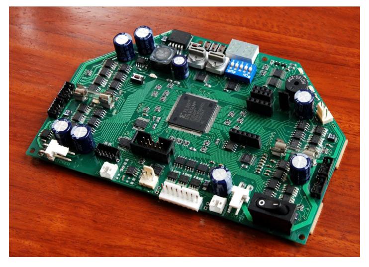
The main electronics board was built last year and we put a lot of components on it but some of them weren't used such as current sensors. In this year, the new firmware is developed to make the existing components can work fully function.
The board consists of a Xilinx Spartan-3 XC3S400 FPGA, motor driver, user interface, some add-on modules and debugging port. The microprocessor core and interfacing logic for external peripherals are implemented using FPGA in order to handle the low-level control of the brushless motor such as velocity and position control. The main electronics board receives commands from the main software on a computer. The board integrates the processing components together with the power components to keep the board compact and minimize wiring. With limited space, almost components are in small SMD packages. However, these components still large enough for hand soldering with conventional tools. Figure 1 show the main electronics board of the robot.
2.2 Battery and Power Supply
Each robot uses 4-cell lithium polymer battery with capacity around 1700-2200mAh as a power source. The robot can run for several hours with these batteries. There are three main power lines in the robot: kicker board, motor driver and processing components. These lines are fused with different current rating fuses. The power supply current is monitored by the current sensors which are attached to each motor driver and kicker board to limit the current when short-circuit occurs.
2.3 Motors
There are two types of motor in the robot, the driving motor and the dribbling motor, both are brushless motor. Each driving motor is a 30 watts Maxon EC45 flat motor with a custom back-extended shaft for attaching encoder wheel. The motor itself can produce a feedback signal from hall sensors for measuring wheel velocity. However, this multi-pole motor sends only roughly 48 pulses per revolution; therefore, this motor is needed to be attached by an US Digital E4P encoder which have higher resolution of 1440 pulses per revolution. The dribbling motor is a high speed 15 watts Maxon EC16 motor. Despite a very low resolution of 6 pulses per revolution signal from hall sensors, the implementation of the PI control law is possible when using this motor at high speeds. The dribbling bar maximum speed is about 13000 rpm.
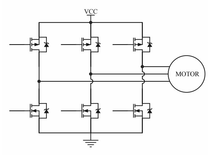
The motor driver is a three phase inverter circuit using complementary N and P channel power MOSFET in each phase. This configuration doesn't require bootstrap driver as in N channel only configuration. These MOSFETs are driven by MOSFET driver ICs to minimize switching loss. The motor commutation and PWM generation are described in the firmware section. Figure 2 shows the three-phase brushless motor driver circuit.
2.4 Kicker
Both kicker and chip kicker in the robot are energized by solenoids. These solenoids are fed with a high current impulse to produce intense magnetic field in a short period of time. The impulse current is created from discharging the high voltage capacitor into solenoid wire. Charging and discharging the capacitor are controlled by the kicker board. This board consists of power switching devices: MOSFET and IGBT which are controlled from the main board.
The charger is a switching DC boost converter circuit. The RC snubber is added into the switching node in order to reduce ringing and EMI which are created by the parasitic inductances and capacitances [2]. Last year, we used a large toroidal inductor in the charger which can withstand a high current without overheating. This year, we use the smaller SMD inductor with the same current rating. However, this inductor has a lower inductance so we need to increase the switching frequency. With current design, the kicker board can charge two 2700 µF capacitors from 0V to 250V in about 5 seconds with 2A average current.
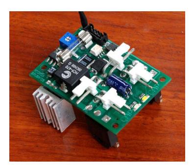
The kicker is a cylindrical shaped solenoid attached to a curved kicking plate and the chip-kicker is a flat shaped solenoid attached with a 45 degree hinged wedge. These solenoids are driven by IGBTs and the kicking force is controlled using PWM signal. The kicker board is depicted in Figure 3.
2.5 Sensors
There are several local sensors to get some helpful information from the robot. The infrared break beam in front of the kicker is used to detect the presence of the ball. This sensor is useful in the passing and one-touch shooting skills that use this sensor as a trigger for the kicker because the vision cannot detect the ball location accurately. We are also developing another infrared sensor which uses an array of infrared emitters and detectors to detect the ball position relative to the robot, so the robot can localize itself more accurately rather than using only the vision when receiving or approaching the ball.
2.6 Communication
The communication between robots and the server can be made by using a radio device. A bi-directional wireless module is operating at 2.4GHz frequency in ISM band which offer channel switching around 2.4GHz to 2.5GHz for the communication. These modules consist of some variants of wireless transceiver ICs from Nordic Semiconductor: nRF2401A, nRF24L01 and nRF24L01+. Despite the modules with lower frequency have longer range and lower interference, some of them aren't permitted in some region.
Each robot communicates with an external wireless board which is linked to the computer via a USB port. This board consists of two independent wireless modules which can provide a full-duplex communication.
2.7 Debugging
The main board has switches, LEDs and buzzer to provide debugging capabilities. These components are connected to the FPGA using shift registers to minimize FPGA input/output pins so in this case only four signal lines are used. The robot can perform several tests for calibrating and setting parameters such as the kicker force and sensor compensation without using any commands from the computer. These parameters are also saved inside an onboard non-volatile memory. This memory also used as storage for capturing encoder, current or other information which can be downloaded via a serial port. This information is very useful for PI controller tuning and sensor calibration.
3 Robot Firmware
The main electronics board consists of a FPGA as a single chip central controller. The FPGA is embedded with a 32-bit processor, brushless motor controller, PWM generator, quadrature decoder, kicker board controller and onboard peripheral interfacing cores: SPI and UART. The processor runs at 30MIPS as same as oscillator clock speed. We use Altium Designer and Xilinx ISE software to generate, configure and debug these cores.
3.1 Brushless Motor Driver
The three phase inverter bridge is fed with signals from FPGA to provide commutation for each motor. These signals are ANDed with the PWM signal to vary the average voltage applied to the motor winding. The six steps commutation sequence is detected by three hall sensors in the motor.
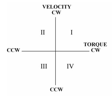
Last year, we kept the high side driver turn on for each commutation step and send the PWM signal to the low side driver only. We found a crucial problem caused by this approach [3]. The motor runs normally in quadrant I and III which torque and velocity are in the same direction (the motor is accelerating). When operating in quadrant II and IV (the motor is braking) the high side driver shorts the motor's back EMF in every commutation step, creating a reverse torque. This torque cannot be controlled as it's from the high side driver which is fully turned on for each commutation step.
This problem can be solved by sending the PWM signals to both high and low side drivers. As shown in Figure 5, the motor velocity are observed when the motor is accelerating and braking. The blue line indicates desired motor velocity and the red line indicates actual observed velocity. The problem is solved by using new PWM method and the motor runs smoothly both accelerating and braking. These two results are captured from one of the robot motor controlled by a properly tuned PI controller with no load. Note that the deceleration in the lower chart is higher than the upper one.
3.2 Motion Control
The robot employs a PI controller as a motion controller, one controller for each motor. The control loop executes 600 times per second using velocity feedback from the encoder in driving motor and hall sensors in dribbling motor. The proportional and integral gains are manually hand-tuned. The computer sends a velocity for each DOF: x-y axis and rotation axis. Then, converted to each wheel velocity and sent to the PI controller. In order to control the motor, the dynamics of the motor has to be modeled first. The dynamic equation for the Maxon brushless motor can be described as [4]:
$$u \cdot \frac{\tau_m}{k_m} = \frac{\pi}{30,000} \cdot \dot{\phi} \cdot \tau_m + R \cdot \left(\frac{\tau_m}{k_m}\right)^2 \tag{1}$$
where:
$u$ is the input voltage
$\tau_m$ is the motor output torque
$k_m$ is the motor torque constant
$\dot{\phi}$ is the motor angular velocity
$R$ is the motor coil resistance
Equation (1) is not easy to be directly implemented to the robot; therefore, this equation has to be modified by using the Maxon parameters relationship, which is shown in its datasheet, and the final dynamic equation of the motor is
$$\tau_m = \left(\frac{k_m}{R}\right) \cdot u - \left(\frac{k_m}{R \cdot k_n}\right) \cdot \dot{\phi} \tag{2}$$
where:
$k_n$ is the motor speed constant
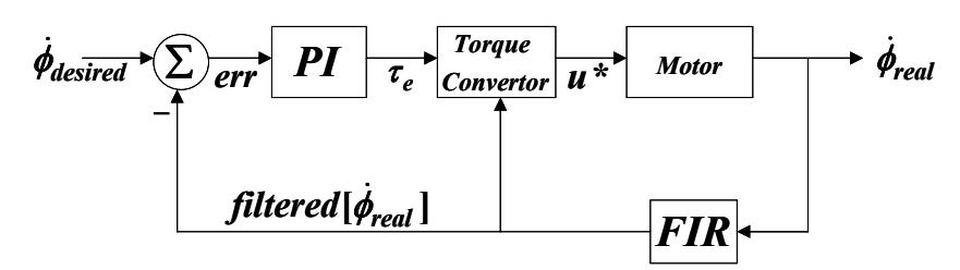
This equation shows that we can control the output torque of the motor at specific angular velocity by control the control signal u. The control law is set using the discrete Proportional-Integral control law and torque dynamic equation (2). The control system runs at 600Hz cycle. The error between desired angular velocity and real filtered angular velocity of each wheel is the input of the PI controller with the PI gains $K_p$ and $K_I$ respectively. The controller is shown in Figure 6 and the control law can be described as (3) through (5).
3.3 Over-current Protection
General problem when driving the inverter bridge is the shoot-through current. This current is caused by turning on one side driver immediately after turned the other side off as the MOSFET turn-off time is usually higher than the turn-on time. This situation occurs when the motor is reversing direction, which can be prevented by adding a small delay time between each high and low side driver signal.
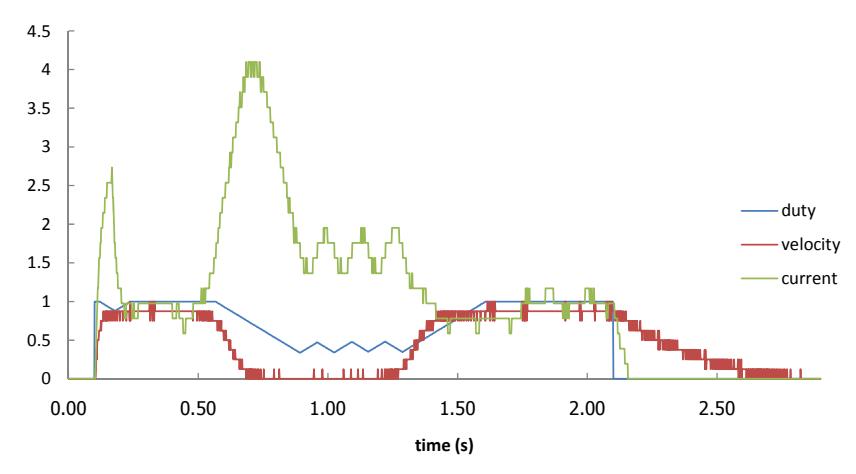
In this year, many robot skills are relied much more on the dribbler. Some ball stealing skills can cause dribbling motor to stall when the dribbling bar is contacted with the opponent robot. The stalled motor consumes very high current and often burn the fuse out. This over-current situation can be detected by a current sensor and can be prevented by limiting a PWM duty cycle until the current drop below the safe motor operating current. Figure 10, depicts the motor stalling situation. When the motor stalled, the motor current increased and dropped in a short time due to limited duty cycle. The motor current are controlled around the limited threshold while the motor is stalling.
3.4 Kicker
Kicker board consists of power electronic components which are controlled directly from the FPGA in the main board. The board requires PWM signal for switching circuit and another PWM signal to impulse the kicker with the desired kicking force. The switching DC converter uses a soft-start method to reduce inrush current when the capacitor is empty. This method is done by starting with the low duty cycle and ramping up over the time until it reaches the limit. The ramping starts again when the kicker is activated. Details about operation and implementation of a similar circuit are in [5].
3.5 Infrared Sensors
The robot uses a pair of infrared break beam. The infrared detector signal is compared with the threshold level and outputs a digital signal to the FPGA.
In addition, an array of infrared emitter-detector pairs is used to detect the position of the ball in a very precise value compared to the vision. However, operating these two types of infrared sensors in the same time will cause infrared light to interfere with each others. The robot runs the calibration first, by reading sensor values when all of the emitters are turned off to get the ambient values. Then, each type of the emitter turns on and off sequentially to read the value for each sensor. The later readings are subtracted with the ambient readings to obtain only the sensor values. Each infrared emitter can be driven from very high current up to several hundreds of milliamperes using this method due to very short period of turn-on time. This high current capability improves the range and signal to noise ratio for the detectors. The sensor data interpretation method is currently still in development.
3.6 Communication
The robot commands are sent to each robot for each frame of software execution. Then, each robot sends back the status after received its commands immediately. The commands are in small packet containing velocities, dribbler and kicker command with some headers for testing and calibrating purpose. The robot status contains a battery level, current consumption and sensors information.
4 Robot Mechanical Design
This section describes the mechanical system of the robot which consists of the driving system, ball control system and kicking system. In RoboCup 2008, we experienced the problem with many parts of the robot and they are the guideline to our development in this year.
4.1 Wheels
Skuba robot uses an omni-directional wheel for the first time in Skuba 2005 model. This robot has only three wheels. Skuba 2006 model uses four omni-directional wheels rather than three wheels in order to get more speed and acceleration. Each wheel is made from aluminum with thirty small rollers. Although the robot can make the smooth motion, it still has a lot of slipping.
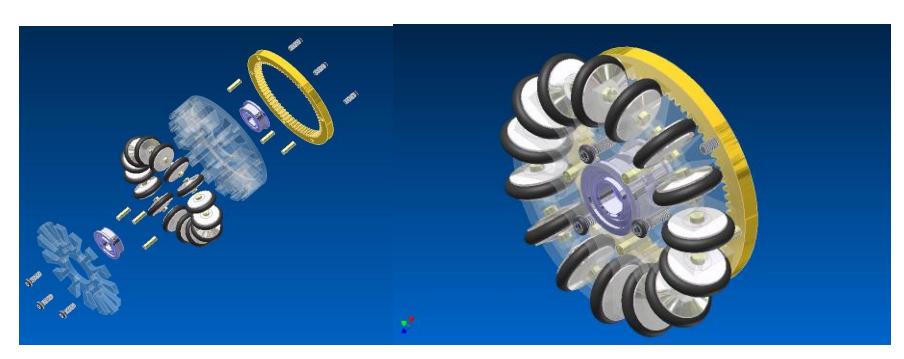
Skuba 2009 robot uses four omni-directional wheels. The wheel has a diameter of 50.8 mm which its cover is made from aluminum and its base part is made from polycarbonate, the light weight material, with fifteen rollers. Double seal o-ring is used for each roller in order to get more friction. All of these components, leading to the light weight and better tracking wheel and finally we have a light weight and better robot. We use pins to fix the position between the cover and the base to reduce the positioning error. This wheel makes robot moving with higher acceleration at approximately 3.5 m/s² and higher velocity at approximately 5 m/s. These values are the maximum controllable velocity and acceleration that the robot can provide. The Skuba 2009 wheel is shown in Figure 11 (CAD model) and Figure 12 (real wheel).
4.2 Driving System
The previous robot models (Skuba 2006 and Skuba 2007) used Faulhaber 2224 motor with the gear ratio of 14:1. We applied the voltage of 12V to the motor that is limited to 6V. Thus we encounter with a trouble of overheating and burning out. This motor can produce acceptable moving speed at that moment but for now, it requires more velocity and acceleration to make the robot more competitive.
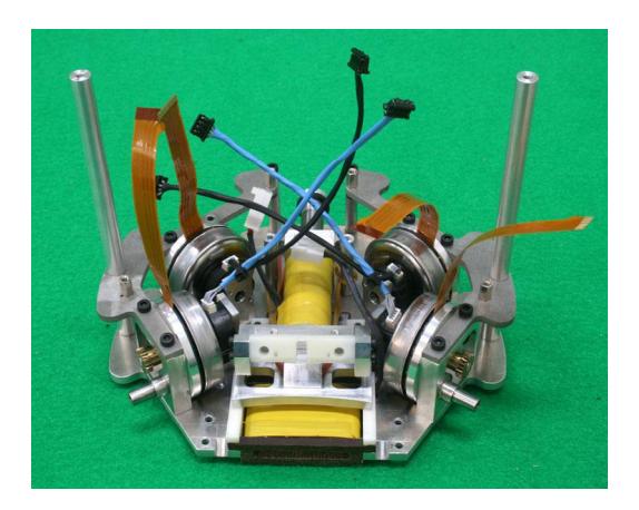
Skuba 2009 robot uses brushless motor, 30 watts Maxon EC45 flat, in the driving system which can produce a lot of torque and more robust than the previous model. The driving system uses gear ratio of 3.60:1 (72:20). This is the proper ratio to get the satisfying acceleration and velocity with the specified wheel diameter. Another reason to choose this motor is its lower price than the previous model. The 5 mm-thick bottom plate connects all of the robot parts together. The robot's partly assembled chassis is shown in Figure 13.
4.3 Ball Control System
(Section header)
4.3.1 Suspension System
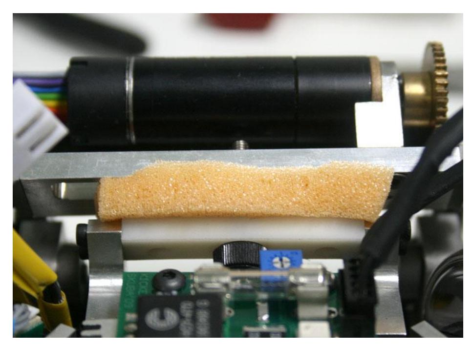
In Skuba 2008 robot, it is the first time that we applied the suspension system to the robot. It is a swing suspension hinged with the chassis plate which is attached with a sponge damper. We use adjustable screw as the stopper, allowing the suspension swing about 6.5 degree. This suspension system makes the robot able to receive the fast moving ball in passing skill.
This year, we develop a new suspension system using the stronger material, stainless steel, and design a firmly structure which result in the more robust system than the previous model. Furthermore, both outer sides of the suspension arms are equipped with the covers to protect the infrared sensors from damaging. Figure 14 shows the suspension system of the Skuba 2009 robot.
4.3.2 Dribbling System
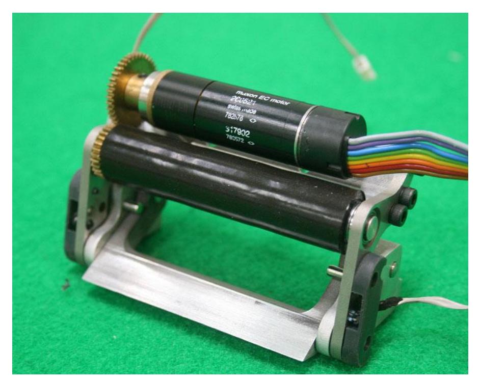
Suspension and dribbling system are both necessary for controlling the ball. In Skuba 2009 robot, 15 watts Maxon EC16 is used as a dribbling motor. It can produce high torque and speed. The gearhead is attached to this motor. The dribbling bar can spin at the maximum speed of 13000 rpm. The dribbling bar is made from aluminum rod with diameter of 10 mm as shown in Figure 15. The dribbling bar is covered with a silicone tube which has a good property to drib the ball. Although this material is good but sometimes it cannot grab the ball; thus we will try to find the better material that has more flexibility. Both suspension and dribbling system are designed with respect to the rules.
4.4 Kicking System
(Section header)
4.4.1 Kicker
The kicker is energized by solenoid system. It is the cylindrical solenoid wound with seven layers of 23AWG enameled wire. The kicking plunger rod is separated into two parts. The first part is magnet part which is made from steel and the second is made from material with no magnetic property, aluminum. Both rods have the diameter of 11 mm. These rods are joined together and attached with the curved aluminum kicking plate. This plate has a contacting radius of 300 mm which results in more accurate shooting when the ball is not in the center of the kicker. The kicking system makes the robot able to kick the ball at maximum speed of 12-14 m/s.
4.4.2 Chip Kicker
In Skuba 2008 robot, it is the first time that we use the new platform of the chip kicker, a flat shaped design. We encounter with many problems such as: unstable, accuracy. Although it has many problems, it still provides lot of advantages. This platform needs smaller area and makes robot more stable due to the lower center of mass. This year, the chip kicker is improved by using original platform of Skuba 2008 model.
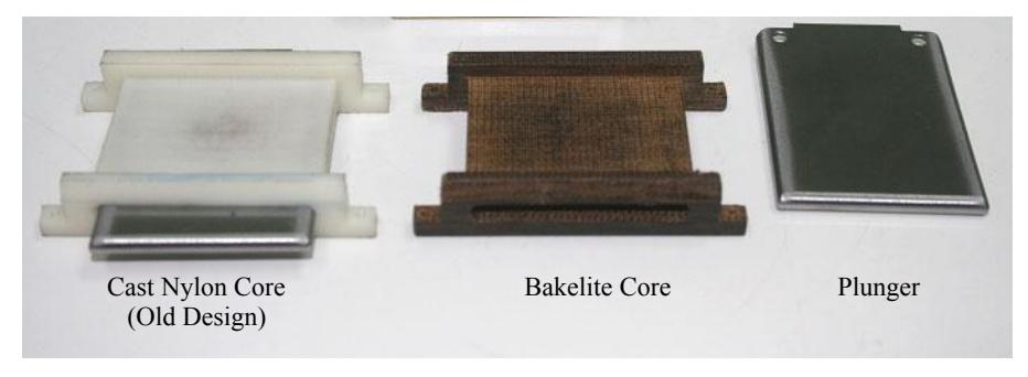
The chip kicker uses the flat solenoid which is the fiber reinforced Bakelite wound with four layers of 22AWG enameled wire. This solenoid is placed in the front part of the bottom plate. The flat plunger is steel with the thickness of 3.75 mm.
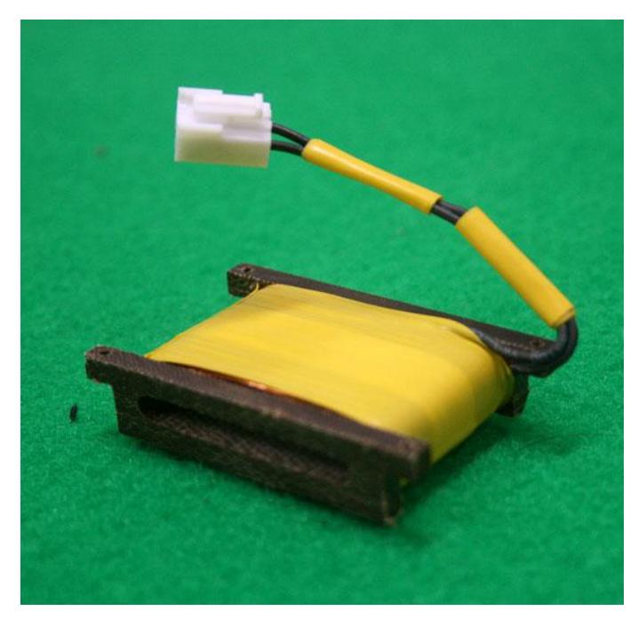
The chipper is a hinged wedge which swings around the pivots. Pin is used as a pivot rather than the bearings because it has more endurance. The swinging degree is also limited by the other pins. The chipper is redesigned and made by one piece 7075 aluminum alloy, which has extra more strength than the standard aluminum. It has a 45 degree slope at the front as the contact point. This chip kicker has an ability to chip the ball with a maximum distance of 7.5 m. Moreover, this chip kicking system is more stable, accurate and robust than the old one. This new design and new material make the robot performs excellent chip kicking action. The chip kicker components are shown in Figure 16 and Figure 17 shows the chip kicker solenoid.
4.4.2 Chip Kicker (continued)
(Continued from chip kicker)
4 Hardware Comparison Table
After combining the entire robot parts, the complete Skuba 2009 robot is shown in Figure 18. Table 1 shows the comparison of Skuba 2007, 2008 and 2009 robots.
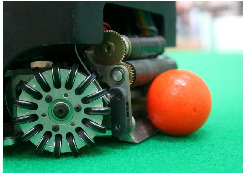
Table 1. Comparison of Skuba 2007, 2008 and 2009 robots.
| Specification | Skuba 2007 | Skuba 2008 | Skuba 2009 |
|---|---|---|---|
| Weight | 2.35 kg | 2.10 kg | 2.30 kg |
| Material | Aluminum | Aluminum | 6061 Aluminum alloy |
| Driving Motor | Faulhaber 2224 | Maxon EC45 flat | Maxon EC45 flat |
| Motor Power | 6 watts | 30 watts | 30 watts |
| Gear Ratio | 14:1 | 3.6:1 | 3.6:1 |
| Max Velocity | 2 m/s | 3.5 m/s | 3.5 m/s |
| Max Acceleration | 2.5 m/s² | 3.5 m/s² | 5 m/s² |
| Wheel Material | Aluminum | Polycarbonate | Polycarbonate |
| Wheel Diameter | 62 mm | 50.8 mm | 50.8 mm |
| No. of Rollers | 30 | 15 | 15 |
| O-ring Type | Round | Round | Double seal |
| Dribbling Bar | Stainless steel, 3 mm | Aluminum, 10 mm | Aluminum, 10 mm |
| Dribbling Material | Sponge | Silicone | Silicone |
| Dribbling Motor | Faulhaber 2224 | Maxon EC16 | Maxon EC16 |
| Dribbling Speed | 2500 rpm | 13000 rpm | 13000 rpm |
| Suspension | No | Yes | Yes |
| Kicker Radius | 80 mm | 150 mm | 300 mm |
| Capacitor | 1100μF, 400V | 4400μF, 250V | 5400μF, 250V |
| Kick Velocity | 7-8 m/s | 10-11 m/s | 12-14 m/s |
| Chip Distance | 2.5 m | 3.2 m | 7.5 m |
5 Vision System
Our vision structure diagram is shown in Figure 19. The description is also shown below Figure 19.
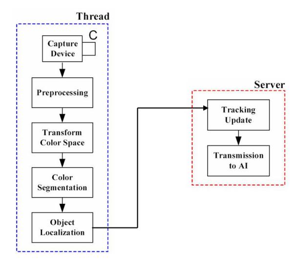
5 Capture Device
The Skuba vision system applies the global vision and uses the output signal of two AVT Stingray F-046C 1394b firewire cameras which is capable of grabbing 780 x 580 images at 62 fps.
5 Preprocessing
The preprocessing is used to improve the quality of the image.
5 Transform Color Space
We transform color model to the HSV space, which consists of a hue, a saturate and a value. The HSV space is more stable than RGB space in different light properties.
5 Color Segmentation
The color segmentation assigns each image pixel into color classes. Currently, we classify and segment color by CMVision2.1 library [6].
5 Object Localization
After color segmentation, we receive all the color regions. The filtering process discards incorrect regions. Then, object localization computes the position and orientation of objects in the field from the final regions.
5 Tracking Update
Objects which is received from localization has a lot of noise, so we need to track it. Our approach is working by the Kalman Filter.
5 Transmit to AI
This component consists of network link communication between the vision system and system
5.1 Camera Calibration
Camera calibration is a part in Object localization. We compute the internal and external parameters of the cameras using the Tsai [7] algorithm. These parameters are used to correct the distortion produced by the camera lenses.
6 AI System
Our AI system has been written in C++ and C# language. All software environments were developed under Microsoft Visual Studio 2008.
6.1 Overall Loop
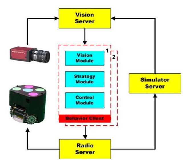
Our system runs exactly 62 times per second equal to camera framerate. Figure 20 shows our overall execution loop.
6.2 VisionServer
The integration of all cameras' information is done on the VisionServer process. The information from two cameras which come from different partially overlapped regions is integrated. Some redundant information is presented. Each information is tagged with the confident value based on confident rules. When the information from two cameras are inconsistent, for example when there are more than one of the same type of object from different camera, the server decides on the highest confidential information. Finally, the vision server sends the consistent information of the whole situation to the BehaviorClient.
6.3 BehaviorClient
The BehaviorClient has three main modules. At the First VisionModule receives vision information from VisionServer or SimulatorServer and predicts that information to account for latency. Then StrategyModule gets predicted vision information from the VisionModule and chooses destinations for all 5 robots. Finally ControlModule retrieves predicted vision from VisionModule and destinations from StrategyModule and makes robots go to those destinations.
6.3.1 VisionModule
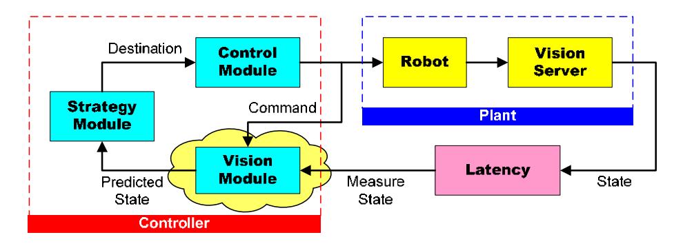
This module was liable for taking the vision data, extracting velocity information from it, and predicting the location of the robots and the ball in the future frame.
Our total system latency, measuring from the period between command velocity and raw velocity, was approximately 133 ms (8 frames). When our robot move at the fastest speed, that is up to about 3.5 m/s, the distance between real robot position and the robot position from vision data will grow up about 47 cm. In order to correct this error we have to estimate the positions and orientations of the robots. The estimation architecture is shown in Figure 21.
6.3.2 StrategyModule
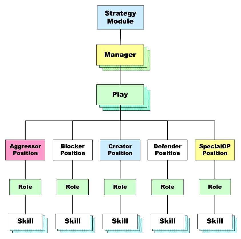
We have a hierarchical model in our StrategyModule design. The module is rebuilt from scratch by using strategy structure based on Cornell Big Red 2002.
The StrategyModule consists of multiple Plays. Whenever a Play is executed it calls the Roles for all Positions present. Then Roles run Skills for the related robots. All the plays are stored in the PlayBook in an array, while all the skills are stored in each SkillSet array.
The StrategyModule architecture is depicted in Figure 22. There are five layers, described in detail below.
6.3.3 ControlModule
ControlModule receives predicted vision from VisionModule and destinations from StrategyModule and makes robots go to those destinations. So, the essential component of ControlModule is a path planning algorithm.
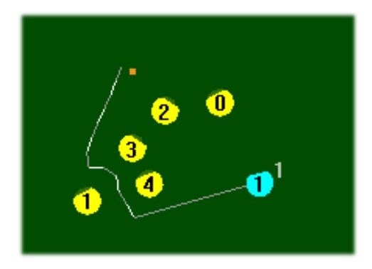
Since the World RoboCup 2008 at Suzhou, we have made use of the "Real-Time Randomized Path Planning for Robot Navigation" [9] for default path planning algorithm. The path planning developed representation on Rapidly-Exploring Random Trees (RRTs) as shown in Figure 23.
6.3.4 Modified Robot Kinematics
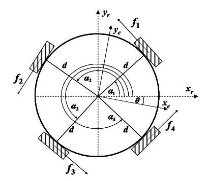
Robot kinematics can be regularly used to generate the path, but in order to make the path more realistic, the dynamics have to be concerned [10], [11]. Although the dynamics can be correctly used to predict the robot behavior but it is hard to be directly implemented to the system and it needs a long computation time. Therefore, the modified robot kinematics is introduced here. Skuba robot chassis is shown in Figure 24 and its kinematics is equation (6).
6.4 RadioServer
Commands which are generated from two individual StrategyModules are encapsulated into a single packet in the RadioServerModules. After commands are packed, the module will send this packet to the wireless board via a USB port. This year, we use full duplex communication for our system in order to get some information form robots in real-time. Therefore, this RadioServerModule is also used to receive the send-back data and return it to each StrategyModule.
6.5 SimulatorServer
Our SimulatorServer is developed in order to simulate robot hardware behavior. The SimulatorServer receives a sequence of packets which is identical to packets that are sent to real robots then calculates some simple physics and returns the coordinate of objects in the field to the software as same as the VisionServer does. Our SimulatorServer is entirely independent from AI System which is capable of simulating all the field objects and latency of the system.
The field objects are simulated by physics engine library called Open Dynamics Engine (ODE) [12]. The SimulatorServer provides connection socket for some two AI systems which means that the simulator is capable to simulate a real competition situation.
7 Conclusion
The new hardware design and the new low level motion controller have implemented and they improved the speed, precision, and flexibility of the robots. With some filters, we could acquire precisely coordinates of all players. The modified robot kinematics is used in the simulator and in the real robot. It can improve the robot overall efficiency. We believe that the RoboCup Small-Size League is and will continue to be an excellent domain to drive research on high-performance real-time autonomous robotics. We hope that our robot performs better in this competition than the last year competition. We are looking forward to share experiences with other great teams around the world.
References
- Srisabye, J., Hoonsuwan, P., Bowarnkitiwong, S., Onman, C., Wasuntapichaikul, P., Signhakarn, A., et al., Skuba 2008 Team Description of the World RobCup 2008, Kasetsart University, Thailand.
- Falin, J.: Minimizing Ringing at the Switch Node of a Boost Converter, Application Report SLVA255, Texas Instruments, September 2006.
- O'Connor, John A.: DEDICATED ICS SIMPLIFY BRUSHLESS DC SERVO AMPLIFIER DESIGN, Application Note, Unitrode Co., Ltd., 1999
- Maxon motor, Key information on maxon DC motor and maxon EC, Maxon Motor Catalogue 07(pp. 157–173), 2007.
- Fosler, R.: Generating High Voltage Using the PIC16C781/782, Application Note, Microchip Technology Inc., 2005.
- Bruce, J.: CMVision realtime color vision system. (The CORAL Group's Color Machine Vision Project) http://www.cs.cmu.edu/~jbruce/cmvision/.
- Tsai, R.Y.: A versatile camera calibration technique for high accuracy 3D machine vision using off-the-shell TV cameras and lenses, IEEE Journal of robotics and Automation, 1987.
- Proving Predictive Control of a Mobile Robot:Application of Image Processing and Kalman Filtering, IMTC 2003, Instrumentation and Measurement, Technology Conference, CO, USA, 20-22 May 2003.
- Bruce, J.; Veloso, M.: Real-time randomized path planning for robot navigation, Intelligent Robots and System, 2002. IEEE/RSJ International Conference on, Volume 3, 30 Sept.-5 Oct. 2002 Page(s):2383 - 2388 vol.3, 2002.
- Oliveira, H., Sousa, A., Moreira, A., Casto, P., Precise Modeling of a Four Wheeled Omnidirectional Robot, Proc. Robotica'2008 (pp. 57-62), 2008.
- Rojas, R., Forster, A., Holonomic Control of a robot with an omnidirectional drive, Kunstliche Intelligenz, BottcherIT Verlag, 2006.
- Open Dynamic Engine, http://www.ode.org.