Extended TDP of ZjuNlict 2009

Yonghai Wu, Xingzhong Qiu, Guo Yu, Jianjun Chen, Xuqing Nie, Rong Xiong

National Laboratory of Industrial Control Technology Zhejiang University Zheda Road No.38, Hangzhou Zhejiang Province, P.R. China

http://www.nlict.zju.edu.cn/ssl/WelcomePage.html

Abstract This paper summarizes the details of ZjuNlict robot soccer system we have made since participated in Robocup2004. In this paper we will emphasize the main ideas of designing of robot subsystem, vision system and AI system. Also we will share our tips in some special problems.

1 Introduction

Our team is an open project supported by the National Lab. of Industrial Control Technology in Zhejiang University, China. We have started since 2003 and participated in RoboCup 2004 2008. The competition and communication in RoboCup games benefit us a lot. In 2008 Robocup, we were one of the top four teams of the world. We also won the first place in Robocup China Open 2008, and are now the champion team of China.

Our Team members come from serveral different colleges, so each member can contribute more to our project and do more efficient job.

Team Leader Yonghai Wu (AI) Team Member – Xingzhong Qiu(AI)

• Zhonghao Huang(Vision)
• Jianjun Chen(Electronic)
• Xuqing Nie(Mechanics)

2 Hardware Architecture

[This section contains subsections]

2.1 Hardware of Vision System

We use two Basler A310a Fireware cameras with TAMRON len, whose focal length is 4 12mm , one for each half field. The image data is sent through 1394 FireWire to PC at the speed of 60f /s and the resolution of the image data is 640 × 480.

2.2 Robot

[This section contains subsections]

Components of the Robot

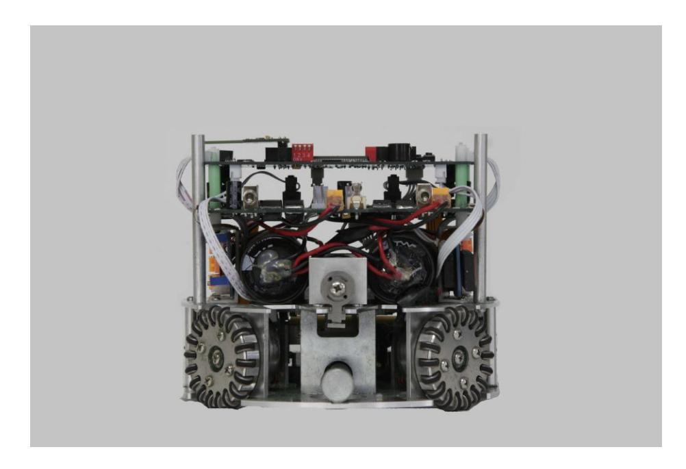
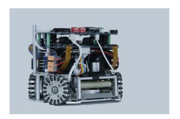
Our robots are equipped with 4 omni-directional wheels. Each is driven by a 30 watt brushless Maxon motors which help our robot run with about 2.5m/s and 6.0m/s$^2$ . The reduction ratio of the gearbox with internal spur gear is 4:1. Besides there are three major machinery devices: a dribbling device, a shooting device and a chipping device. The robot is shown in Figure 1

Mechanical Design

[This section contains subsections]

Omni-directional Wheel Design

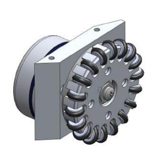
Each wheel is composed of a big aluminous wheel with 18 grooves distributed equably in Circle, there is a small wheel founded with PM in every groove. Similarly, there is a groove in the small wheel, covered by a o-ring. The omni-directional wheel is shown in Figure 3 In Robocup 2008, the wheel exhibited some problems, such as large gap and friction. Now the wheel is redesigned in some details, and receives a perfect performance. Except the wheels, we do not change a lot in the other parts. To improve the manufacture precision, we make all the parts with CNC machine tools.

Shooting Device Design

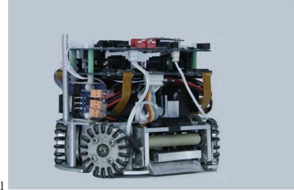
The robot's shooting device is the primary method of both scoring and passing. It is made up of a an electromagnet and a simple mechanical structure. The electromagnet is made by ourselves and is calculated accurately in advance. It is drive by two big capacitors which is fixed on the floor board above. Since nn Robocup 2007, we are pleased with our shooting devices and don't change a lot. It is shown in Figure 4. The shooting device can give the ball a maximum velocity of 11m/s. In the match, it is controlled by the circuit, the time and the force of kicking the ball is also in charge. This part of the robot is usually cooperate with others, such as the chipper,the dribbler.

Chipping Device Design

The chipping device allows the robots to pass the opponent by kicking the ball into the air. As same as the shooting devices, it is also drive by two capacitors, the method to control it is also the same. It is shown in Figure 5. When the chipping device works, the shovel close to the ground can chip the ball to a maximum height of 0.8m and a maximum

Dribbling Device Design

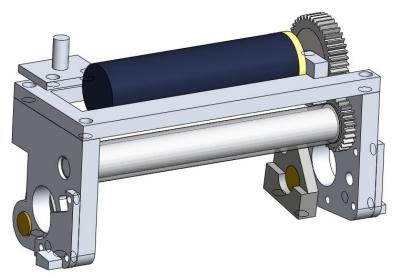
The dribbling device is the assembly that controls the ball. It is designed to stop a ball, control it and prevent losing it. The dribbling device is drive by a motor, accelerated by a pair of gears. A stick swathed with a special pipe circum gyrates when the ball comes close to the robot or it must compete for the ball with the opponent. From Robocup 2006 at Bremen, we found that the ball controlling ability is not very satisfactory, these years, we have tried many ways to improve it. We get a lot of experiences, receive a much better result now. It is shown in Figure 4. The higher rotate speed the motor circum gyrate, the bigger force the ball is given, but on the other hand, the ball will be easier to lose control. To get a better effect, we redesigned the limit device, besides we spend a lot of time choosing the material.

Electronic Design

[This section contains subsections]

Driving Peripheral Design

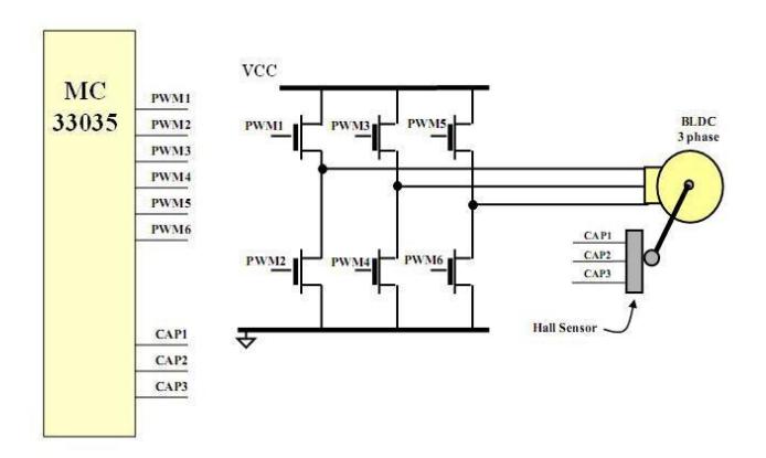
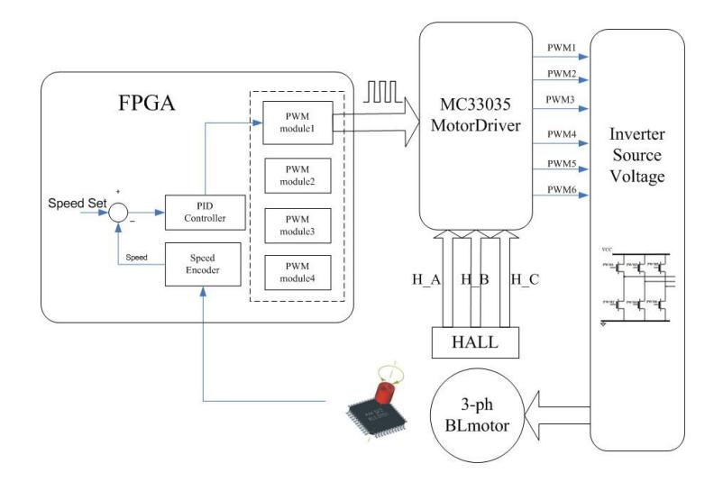
There is a local feedback control loop on the robot. Motor driving module based on MC33035 which consists of a rotor position decoder for proper commutation sequencing, temperature compensated reference capable of supplying sensor power, frequency programmable saw tooth oscillator, three open collector top drivers, and three high current totem pole bottom drivers ideally suited for driving power MOSFETs, Can Efficiently Control Brush DC Motors with External MOSFET H-Bridge.( Figure 7)

Communication Peripheral Design

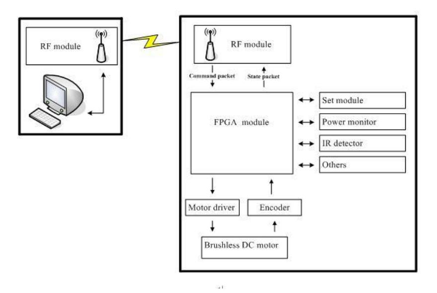
Our communication system is based on the module of NRF2401. NRF2401 is a single-chip radio transceiver for the world wide 2.4 - 2.5 GHz ISM band. The transceiver consists of a fully integrated frequency synthesizer, a power amplifier, a crystal oscillator and a modulator. Output power and frequency channels are easily programmable by use of the 3-wire serial interface. This year, a new communication system has been developed to reach better results. The new communication system is based on two RF modules on the robot. They were two separate modules, respectively charging for receiving and sending. Compared to last year, data transferred from the pc to robot, is encoded to a larger packet. All of the robot on the ground can receives the same packet at the same time, and pick up the right information with the numbers of themselves. the right information picked up from the large packet includes the speed of every wheels, shoot or chip command, the number of robot. Thus, every robot can receive the order without delay. Meanwhile the robots can send a packet to the pc. However, there is only one robot can send packet that contains useful information to pc. The PC can receive information from the robot without any delays. So the command sent from the pc can be implemented more effectively and timely.

Shooting Peripheral Design

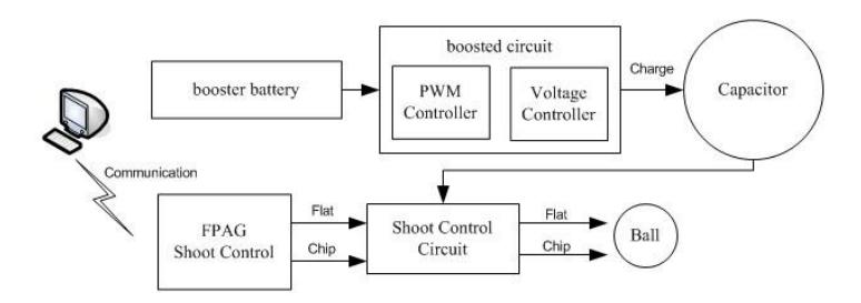
Compared to previous years, our Shooting system ( Figure 8 )is not changed too much this year. Our boosted circuit includes a PWM control module and voltage control module, to control the boost capacitor voltage. FPGA sent chip or flat shoot signal, through control circuit for chip or flat shoot. However, we choose two smaller capacitors with higher voltage, to achieve a better result. The kicks are driven by two 4700uF capacitors charged to 100V. The kicker can give the ball a maximum velocity of 10m/s [3], [2], [4]. With the increased voltage, the velocity will be faster.

3 Software System

[This section contains subsections]

3.1 Emebedded Software

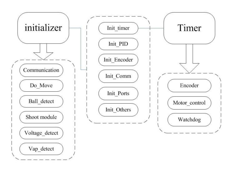
Since Robocup2007 in Atlant, Our circuit architecture use the NiosII as the central processor module which is a soft IP provided by Altera company matching at QuartusII5.1 and NiosII5.1 software programming environment. The overview of our embedded software flow is show in Figure 9

Motor PID Control

Based on our motor driver module ( Figure 10 ), we use an incremental PID algorithm, real-time code set encoding to read the speed of motor for PI and PID control, so that motor speed can reach the stable speed settings. About the encoder module, we use AM512, which is a compact solution for angular position sensing. The IC senses the angular position of a permanent magnet placed above the chip. So we put the permanent magnet on the motor, when the motor rotation, FPGA board will receive the Incremental signal from the encoder module. There are two signals for incremental output: channel A and channel B. Signals A and B are quadrature signals, shifted by 90. The speed of the motor can be count by the signals.

3.2 Vision System

[This section contains subsections]

3.2.1 Calibration

Calibration parameters are computed via Tsais method [5], which is programmed in MATLAB, and are then used to map the object coordinate on the image to the coordinate on the field. The error between the computed field coordinate and the actual one is less than 15mm.

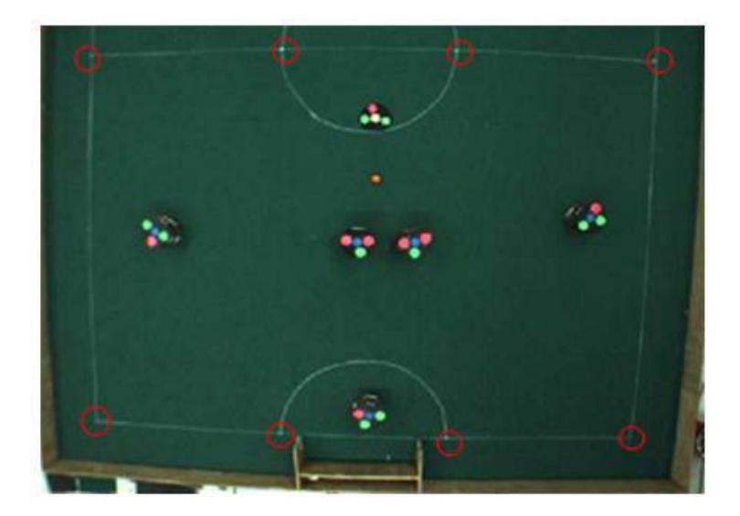
Tsais method for camera calibration recovers the interior orientation, the exterior orientation, the power series coefficients for distortion, and an image scale factor that best fit the measured image coordinates corresponding to known target point coordinates. This is done in stages, starting off with closed form least-squares estimates of some parameters and ending with an iterative nonlinear optimization of all parameters simultaneously using these estimates as starting values. Importantly, it is error in the image plane that is minimized. Details of the method are different for planar targets than for targets occupying some volume in space. Accurate planar targets are easier to make, but lead to some limitations in camera calibration. Besides, figure 11 shows that we choose the 8 points(corner points or intersect points) in the field.

3.2.2 Sampling and Segmentation

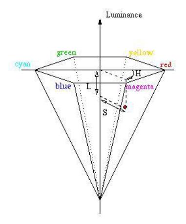
First of all, we use the HSI color model, HSI space are transformations of RGB space that can describe colors in terms more natural to an artist. The two spaces can be thought of as being single cones, as shown in Figure 12. The hue component in the color space is an angular measurement, analogous to position around a color wheel. A hue value of 0 indicates the color red; the color green is at a value corresponding to 120, and the color blue is at a value corresponding to 240. Horizontal planes through the cones in Figure are hexagons; the primaries and secondaries (red, yellow, green, cyan, blue, and magenta) occur at the vertices of the hexagons. The saturation component in color space describes color intensity. A saturation value of 0 (in the middle of a hexagon) means that the color is "colorless" (gray); a saturation value at the maximum (at the outer edge of a hexagon) means that the color is at maximum "colorfulness" for that hue angle and brightness. The I component describes brightness or luminance. A value of 0 represents black. In the space, a maximum value means that the color is at its brightest. Regardless of the current values of the hue and saturation components.

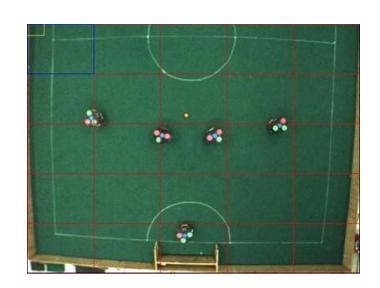
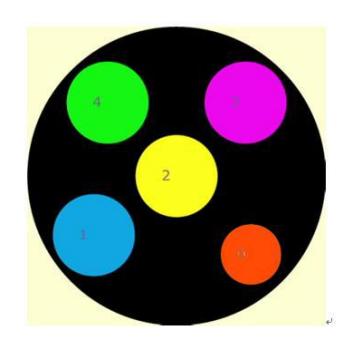
In order to differentiate the various objects on the field, i.e. ball, our robots and opponent robots, first we need to decide the color thresholds for these objects. Considering the inconsistent light condition of the field, we decided to use local thresholds method, which divides the whole field into many blocks, each of which stores its own set of threshold parameters as shown in Figure 13. Moreover, in order to obtain these sets of parameters more conveniently, we designed a cover with special color configuration, which can be worn by our robot and ran over the field so that every blocks threshold data are updated, figure 14shows the cover.

3.2.3 Object Recognition

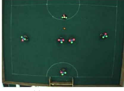
To minimize the computation load, first we take a background image without any objects in it. Then, during processing, the new image minus the background image is changed to HSI color space, and colors on the image are decided using the threshold parameters that previously set as shown in figure 14. Contour tracing method is used to find connecting regions with a same color. Blobs of different colors form a certain configuration enable us to recognize the ball and the robots. After both of half-field images are processed, in accordance with history information and sizes of the blobs, information from these two images are merged to generate our final result.

3.2.4 Blobs Model

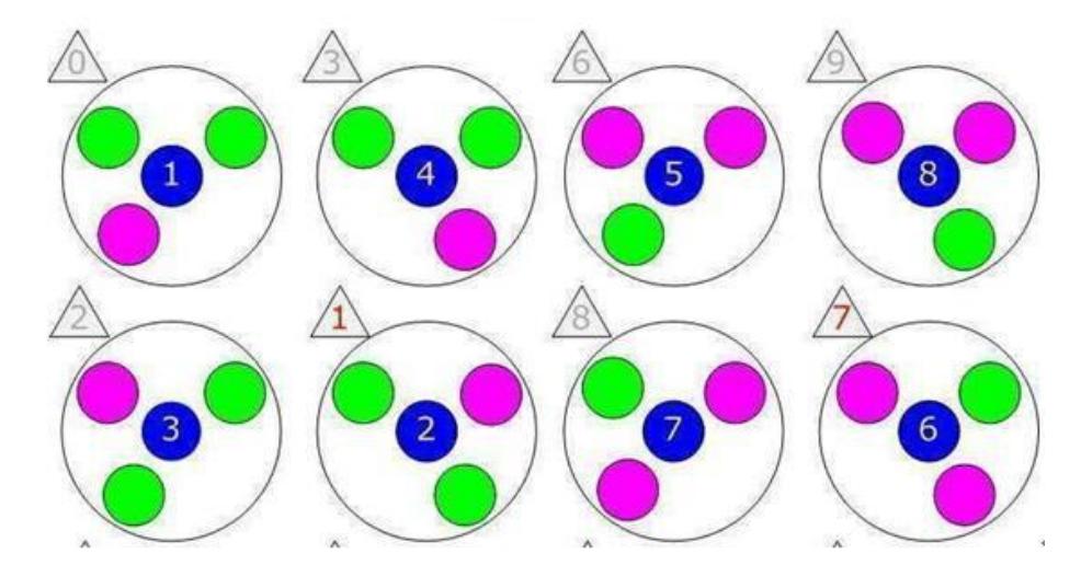
We choose FU model as our blobs model as shown in figure 16. Then we can recognize the direction and id of each robot.

3.3 AI System

The AI system is running on a PC installed Windows Xp. It connects the vision system via UDP, and connects the radio system via serial port. Besides, we have a debug GUI client connecting the AI system via TCP, which uses the same protocol to connect vision system. An ODE based Simulator help us to test some hardware independent algorithms. Our whole software development works under Visual Studio using the C++ language.

3.3.1 Decision Flow

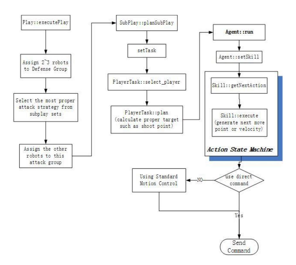
We use a multi-layered learning based play/subplay/agent/skill [6], [1] architecture which of decision routine is show in figure 17, In the Play layer, the most fitness tactic will be selected, then each robot will assign a task. Some task may be very simple such as going to a specific point for receive or block. Some task may be very complex such as shoot goal, which is composed by intercept, grasp ball and aim target etc base skill. We use the finite state machine to link these actions.

3.3.2 Object Prediction

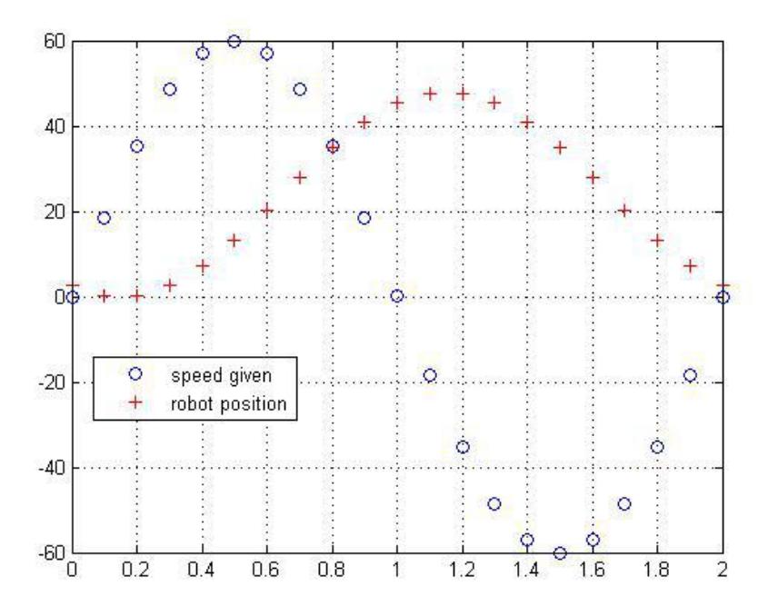
Because of the network transmission and image processing time cost, the AI module generated command received by robot will be later than the time camera captures this frame image. But when making decision we should take account of the state in which the robot just receives the motion command. So we must predict all of objects state in the field such as ball, our member and opponent in this latency duration (Figure 18).

Latency Measurement

In prediction routine, we must first know the system latency which starts in image capture and ends in the time command received by robots. We designed a easy experiment to measure this latency time. Detail of the experiment routine is show in following:

• 1. Make a robot stop in field, log this initial position
• 2. in the frame t we send a direct velocity along x axis which magnitude is k1sin(k2t), where t is the sample (or send) cycle.
• 3. At the same time we log this velocity command and robots new position
• 4. Without system latency, when the command speed accelerate to reach its maximum value, and then decelerate to zero, the robot just moves to the farthest distance away its origin position in positive direction. While command is negative, the robot goes back to its origin position.
• 5. Considering the system latency, when the command is send, it is after some time that robot will receive this command. So the time when command reaches zero doesnt synchronize the time when robot moves farthest.

6. Plot the robot position and command velocity magnitude in figure 18, we can see the difference between the time when the robot moving distance reaches its maximum value and the time when sending speed is zero.

Using this method we can get our system latency is about 4 5 frames (one frame is 1/60 s).

Flying Ball Prediction

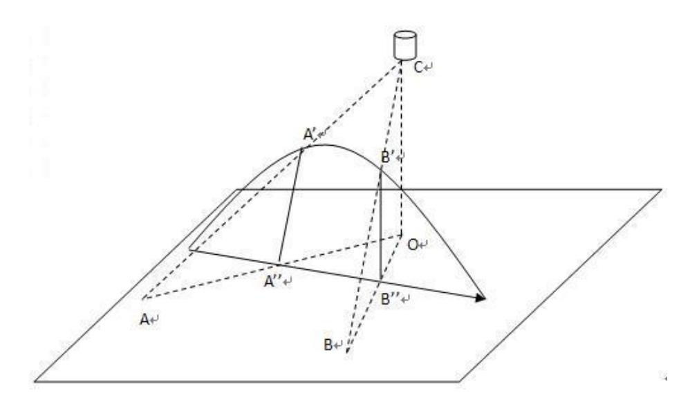
Predicting the flying ball land point is a new topic in small size soccer robot since most teams have robot with chip device. With the chip kicking in cooperation mission we have chance to do the head kicking just like human football game. But in order to implement this, we must predict and calculate the right flying trajectory of ball. Now we share our novel method here.

3.3.3 Path Planning

Path planning is an important issue in the mobile robot domain, we try to find a proper algorithm which can not only reduce the collision between objects more, but also generate a smooth and stable path for the high dynamic environment in robot soccer game. Now we use the A* algorithm to complete an easy but efficient planning model. This path planning algorithm is as follows:

• Step 1 Make certain obstacles which need be avoided according to the robot current position and its desire.
• Step 2 Check the path between start point and target point, and make sure if there is no obstacles along this path. If so, search ends, otherwise go to Step 3.
• Step 3 Create some nodes around each obstacle which can not be ignored.
• Step 4 Using A* Algorithm make search from the start point.
• Step 5 We create an evaluation function to describe the priority of each point in searching procedure.

The first item g(p) represents the distance of this point to start point; The second item e(p) represents the time which robot costs from this point to target point. We use the distance of this point to target to estimate this value; The third item h(p) represents the adaptation of this point considering previous planning result. We have a set to save some way points when a search success. This can accelerate the search procedure if target doesnt change so much. Step 6 In search routine, we always select the point which f(p) value is minimum. Step 7 Check the path between current selected point and other points, if one path is nonblocked, we can add a new edge to the graph, and update the path of the start point to target (this value is initialized to be infinite). This extend method is just like the Shortest Path Algorithm. Step 8 If the path has connected the start point and target point, searching procedure ends, otherwise go back to Step 6. Step 9 Get the first element in generated path to be the robot next move target, and Add the other points to the way points set for accelerate next search.

3.3.4 Behavior Control

[This section contains subsections]

Speed Compensation

Because of the inherent mechanical characteristics, there are variations between the command(|V |, θ, Vrotate) we send to the robot and the result gotten from the execution. These variations are critical in robot motion control. We train a three-layer feed-forward neural network to model the variations, and calculate the compensation we should modify the commands sent to the robots. As for omni-wheels robot, the translation movement and the rotation movement are independent. This means that they can be compensated respectively. We train the neural network in this way: Certain commands(|V |, θ, Vrotate) are sent to the robot, we get the vectors( $(|V|', \theta', V'{rotate})$ ) which robot really executes by measuring the vision logs. For these given commands( $|V|, \theta, V{rotate}$ ):

• -|V| varies between 0cm/s and 250cm/s with a step of 25cm/s
• $-\theta$ varies between 0 and 350 with a step of 10
• $-V_{rotate}=0$

The neural networks [7] input vector is $(|V|, \theta)$ , output vector is $(|V|', \theta', V'{rotate})$ and the hidden layer have 5 neurons. We use the data set gotten in previous measurement to train the network. When the train finished, we get a neural network which can compensate any given command $(|V|, \theta)$ . We also measure the rotate velocity $V{rotate}$ compensation by send commands which $V_{rotate}$ varies between 0rad/s to 10 rad/s with a step of 1 rad/s and |V| = 0. The result show that the Coefficient $\lambda$ compensation for rotate velocity is nearly a constant. ( $\lambda = \frac{V'{rotate}}{V{rotate}}$ ). The compensation of rotate velocity $V_{rotate}$ can be obtained through following equation:

$$V_{rotate}^{''} = \lambda \cdot V_{rotate} + V_{rotate}^{'}$$

$V_{rotate}^{'}$ is gotten by the neural network You can refer to a more detailed method in bibliography

Fetch Ball Control

New approach of fetching a ball is designed with divided states, which cover the situations in procedure of getting the ball. Firstly, the robot moves to the opposite spot of the ball to the target given by a higher layer of the strategy. The path should avoid any possible collision with the ball and get the robot to a final state that staying in line with the ball and target. Then it turns to the next step, GRASP_BALL, the robot keep closing to the ball with a speed depending on the speed of the ball. In this state, the exit condition back to the GOTO_BEHIND is stricter to perform a fluent action. Besides, two different control parameters of the motor are applied for the two steps to get a more accurate and faster response. The following pseudocode describes this decision process.

1 void CGetBallV0::planWayPoint(VisionInformation, ballTarget)
3
   switch (state())
4
   case BEGINNING:
6
       // Variable initalization
7
      setState(GOTO_BEHIND);
8
      break;
9
   case GOTO_BEHIND:
10
       if (isSafeGraspBall and robot, ball and target collinear)
11
        setState(GRASP_BALL);
        break:
     case GRASP_BALL:
13
14
        if (robot, ball and target are non-collinear with buffer)
15
         setState(GOTO_BEHIND);
        else if (ball Controlled)
         setState(FINISHED);
18
19
     case FINISHED: setState(GOTO_BEHIND);
     default: break;
21 }
22}

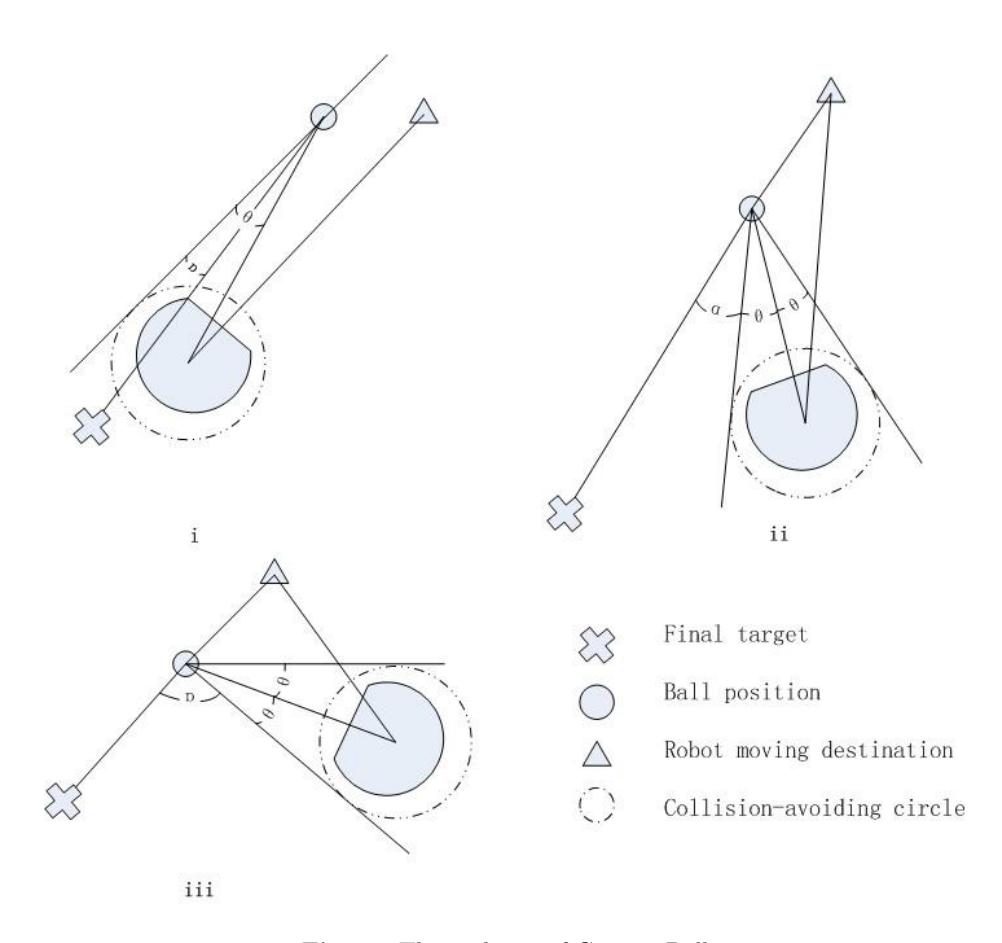
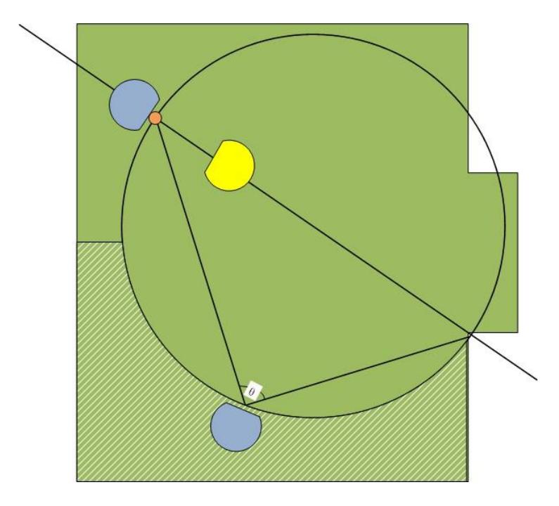
The GOTO_BEHIND state is subdivided into three main situations due to the relative position of the ball, robot and the target. Several veriables are defined to demostrate these relative positions.Let

$$\theta = \arcsin(\frac{r}{|\overrightarrow{m}|})$$

$$\alpha = \pi - \langle \overrightarrow{n}, \overrightarrow{m} \rangle - \theta$$

Where,

$\overrightarrow{m}$ is the collision-avoiding radium $\overrightarrow{m}$ is the vector from robot to the ball $\overrightarrow{n}$ is the vector from the ball to the target

If the robot is in the way between ball and the target ( $\alpha \leq \frac{\pi}{12}$ , figure i), it moves on the line with constant distance to the ball position to avoid blocking the ball. Then if the robot is on the side of the robot (figure ii,iii), it should go behind the ball to get a proper position to push it to the target. The distance d to the ball has a relation with $\alpha$ ; the smaller is the closer robot should approach to the ball. So we got

$$d_0 = \begin{cases} \frac{r}{\sin \alpha}, & (\frac{\pi}{12} \le \alpha \le \frac{\pi}{2}) \ r + 5, & (\alpha \ge \frac{\pi}{2}) \end{cases}$$

Where,

r is the collision-avoiding radius.

K = d$^0$ + dribbleballdist

$\beta$ is the angle between $-\overrightarrow{n}$ and $-\overrightarrow{m}$ , also can be expressed $\langle -\overrightarrow{m}, -\overrightarrow{n} \rangle$

Potential Based Pass and Receive Searching

We have functions to find the best assist point, shoot point or receive point. Several evaluation functions are applied to calculate the rates of each qualified point on the ground according to a set of parameters between ball and goal. As it turned out to cost a lot to recalculate all positions in every cycle,

4 Conclusion

Owing to our all team member hard work, we can obtain this result. If the above information is useful to some new participating teams, or can contribute to the small size league community, we will be very honor. We are also looking forward to share experiences with other great teams around the world.

References

1. Bruce J.R. Browning B. Skills tactics and plans for multi-robot control in adversarial environments. Journal of System and Control Engineering, 2005.
2. Gordon Wyeth David Ball. Uq robocup 2004: Getting smarter. RoboCup 2004, 2004.
3. Ng Beng Kiat. Luckystar 2004. RoboCup 2004, 2004.
4. Aphiwat Kriengwattanakul. Plasma-z 2008 team description paper. RoboCup 2008, 2008.
5. ROGER Y. TSAI. A versatile camera calibration technique for high-accuracy 3d machine vision metrology using -the-shelf tv cameras and lenses. IEEE Journal of Robotics and Automation, 1987.
6. Wenfei Wang. Zjunlict team description for robocup 2009. RoboCup 2009, 2009.
7. Yonghai Wu Yu Sheng. Motion prediction in a high-speed, dynamic environment. Proceedings of 17th IEEE International Conference on Tools with Artificial Intelligence (ICTAI), 2005.