RoboDragons 2010 Extended Team Description
Akeru Ishikawa, Takashi Sakai, Jousuke Nagai, Taro Inagaki, Hajime Sawaguchi, Yuji Nunome, Kazuhito Murakami, Tadashi Naruse
Aichi Prefectural University, Nagakute-cho, Aichi, 480-1198 JAPAN
Abstract This paper describes the system configuration of Aichi Prefectural University's RoboDragons 2010 and related research topics. Main topic in this year is that we developed a new robot hardware. We describe it in detail here. There are some improvements in soccer software. We overview our soccer software. Our research results which will be implemented near future are described: a real time computation of dominant region and a defending strategy based on a safety region.
1 Introduction
This year's extended team description paper (ETDP) of RoboDragons2010 describes a new robot hardware, an improved software of RoboDragons 2010 system and ongoing studies.
First, robot hardware. Our current robots are the fifth generation ones in our Labs. Our team has six robots, five for competition and one for a reserve. Each robot of RoboDragons consists of four omni-directional wheels, a dribbling device, two kicking devices (for chip kick and straight kick) and the embedded computer for controlling the robot. They are controlled by a host computer next to the field. Second, software. The software on the host computer origenates from the one when we made a joint team with CMU in 2004 and 2005. Many improvements have done since 2005, however, this year, noticeable improvement has not done. We overview our software centering on minar changes. Third, research related topics. Several researches on strategies have been doing these years. We introduce the real time dominant region calculation and the defending strategy based on the safety region. These thechneques will be implemented in the RoboDragons system in near future.
In the following sections, we describe these topics.
2 Robots
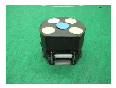
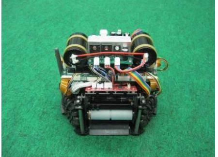
In this section, we discuss our new robots in detail. First, we show the overview of our new robot in Figure 1.
2.1 Dimensions of robot
The robot can be packed in the cylinder with dimensions of 145 mm height and 178 mm diameter. To protect the internal circuit boards and mechanical devices, the robot is covered by the cardboard (see Fig. 1 left). To strengthen the cardboard, the 1.5 mm thick plastic sheet is glued.
2.2 Drive unit
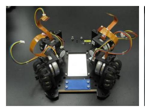
The robot has 4 wheels each of which is drived by a DC brushless motor. The wheel is so called an omni-wheel. Figure 2 shows the omni-wheels moving the robot.
The DC brushless motor driving the omni-wheel is Maxon's "EC 45 flat 30 W" with encoder unit. The source voltage of the motor is 15 V. The motor also has a pinion gear with 21 teeth and the omni-wheel has a gear with 64 teeth so that the reduction ratio is 1 : 3.047. The diameter of the omni-wheel is 56 mm and the omni-wheel has 15 small tires in circumference. The diameter of the small tire is 13 mm.
2.3 Kicking device
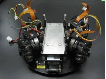
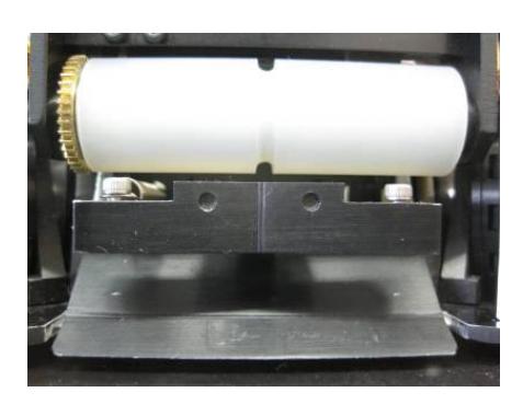
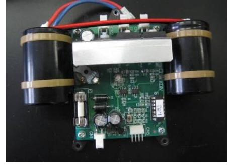
The kicking device consists of solenoids, kick bars, and a voltage booster. Figure 3 (left) shows the kicking device and figure 3 (right) shows the voltage booster.
Solenoids Three solenoids are built in the robot, one large solenoid is for a main kick device and a small solenoid is for a chip kick device.
The coil of the large solenoid is made winding the 0.6 mm enamelled wire on a bakelite cylinder in 7 layers. The dimensions of the cylinder are 13 mm in inner diameter, 26 mm in outer diameter and 55 mm in length. The stroke of the solenoid is 30 mm and enables the kicking a ball with speed of 9.5 msec under the ideal conditions.
The coil of the small solenoid is made using the same material with the large one. The dimension of the cylinder is 13 mm, 26 mm and 27 mm, respectively. The stroke is 7 mm and it can kick the ball with flying distance of 2 m and flying height of 1 m.
Each solenoid employs the spring to pull back the plunger.
Kick bar 7075 aluminum alloy which is light and hard is employed for the kick bar. Moreover, V-shaped ABS plastic is attached to the aluminum kick bar as shown in figure 3. This helps to kick the ball to the direction perpendicular to the kick bar within the accuracy of 5 degree.
Voltage booster: The voltage booster(Fig.3(right)) is a kind of DC-DC converter. It converts 15 V DC input voltage up to 200 V DC output voltage. Output voltage is adjustable between 150 V and 200 V. The chopper circuit using a choke coil is a heart of the voltage booster. A PIC controls the chopper circuit. Large capacity condensers are used for keeping the high voltage output. Total capacity is 4500 µF. The voltage sensing circuit controls the output voltage. 2 solid state relays are used as the switches to drive the solenoids. These relays are controlled exclusively by the PIC. The charging time of the condensers is about 2 sec when the output voltage is 200 V.
2.4 Dribbling device
A dribbling device of the robot has been achieved by combining the dribble roller, the motor and the gear.
The dribbling device uses a Maxon's "EC 16 15W" motor with an encoder and a planetary gear. The reduction ratio of the gear is 1 : 5.4. A pinion gear attached to the motor has 40 teeth and a gear attached to the dribble roller has 36 teeth. Therefore, the net reduction ratio $R$ is given by,
$$R = R_m \times R_g = 5.4 \times \frac{36}{40} = 4.86,\tag{1}$$
where, $R^m$ is the reduction ratio of the planetary gear and $R^g$ is the reduction ratio of the pinion gear and the gear on the dribble roller.
The dimensions of the dribble roller are 20mm in diameter and 73mm in length. The material of the dribble roller is a alminum shaft with silicon rubber of 4mm thickness on the face of the shaft.
2.5 Communication unit
Our wireless communication is a spectrum diffusion communication on the 2.4 GHz band. Futaba's wireless modem "FRH-SD07T" is used for the purpose. The modem has several communication modes. We use a "direct mode" which can send the messages with the least delay between modems. A pair of the FRH-SD03T and the FRH-SD07T realizes the communication between the host computer and the robot(s).
2.6 Proximity sensor unit
The proximity sensor is attached above the dribbling device and it detects the ball just in front of the dribbling device. The heart of the sensor is three infra-red light emission diode (LED) and photo diode pairs. The irradiation angle of the LED is about 15 degree. When one of the three photo diodes gets the reflected infra-red ray more than a preset threshold value, the sensor outputs the signal.
2.7 Control unit
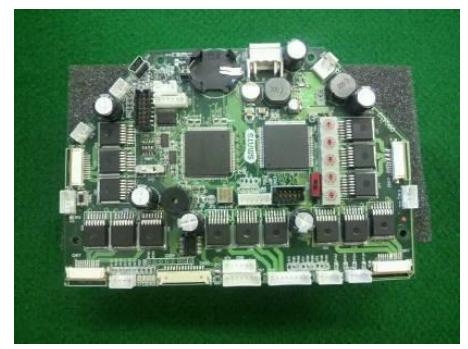
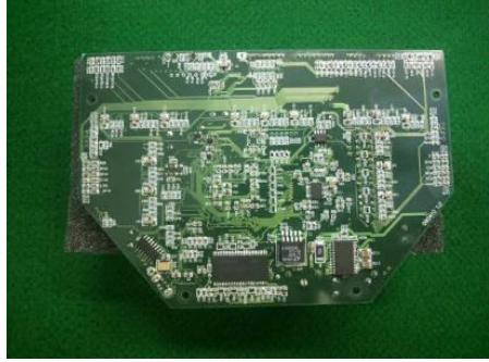
A control unit of robot is a board computer, which is newly developed. It is shown in figure 4 These boards include a The CPU is Hitachi's SH2A processor with FPGA for peripheral control. SH2A has abundant peripheral circuits in it and makes the compact implementation of the control unit possible. The memories compose of Flash ROM(1MB) and SRAM(1MB). The IO boards have power transistors that can drive the motors and they also have interface circuits with the motors driving wheels and dribble roller, and the proximity sensor.
2.8 Control program on robots
At the time this paper is written, the software shown below is not implemented on the robot yet, however, it will be implemented until RoboCup 2010 competition.
The program is written by the C programming language. The TOPPERS real time OS[1] is used.
Robot control program consists of three modules each of which is invoked as a process. They are communication, command and motor control modules. Figure 5 shows a data/signal flow among modules and peripheral units.
Robot command is sent from the host computer to robots by a packet every 1/60 seconds using asynchronous serial communication. Since the communication speed is 19200 bps in our system, it is possible to send 32 bytes data in 1/60 second if only start bit and one stop bit are used as control bits. Therefore, Our packet is consisted of 32 bytes¹ as shown in figure 6. The packet is broadcasted to all robots. The packet has error correcting code (ECC) to make reliable communication possible. We use the Humming code as the ECC.
¹ The command cycle synchronizes with the camera cycle which is equal to 59.94 frames per second. Therefore, the command can send without any problem.
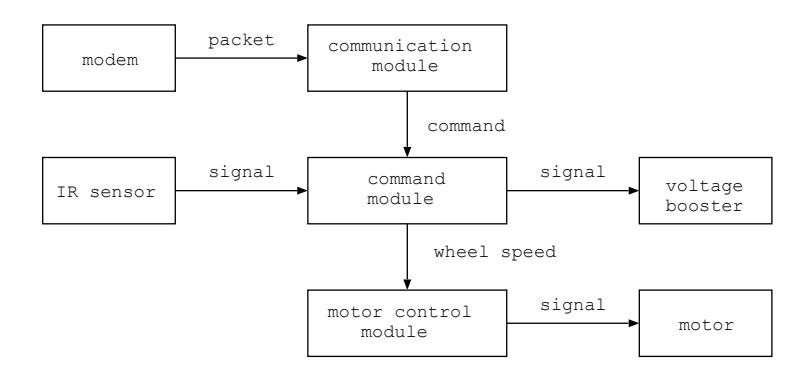
The communication module receives the packet and extracts the command of its own. If error is detected, the packet is discarded. As far as the error is not burst error, the discard of packet is a good alternative². Extracted command is sent to the command module.
In the command module, the velocity of each wheel is calculated from the vel, dir and rot value (see Fig. 6) and calculated result is sent to the motor control module. The kick and dribble command is executed, as well.
In the motor control module, the PID control is performed. This is done by using the target velocity given by the command and the current velocity calculated from the encoder pulses. The motor drive control is done by the PWM control.
² There are no such errors experienced in recent competitions.
class SerialCommand{
 public:
   uint8_t vel; // Velocity [unit: cm/s]
   uint8_t dir; // Direction [unit: 2*pi/256 rad]
   uint8_t rot; // Rotation velocity [unit: 2*pi/60 rad/s]
   uint8_t var; // kick and dribble command
              // b0-b1: kick condition
              // 0 : No kick
              // 1 : kick when center senser reacts
              // 2 : kick when any sensers react
              // 3 : kick immediately
              // b2-b3・b7: Selection of kicker
              // 0 : No kick
              // 1 - 4 : Main kicker (1: weak ... 4: strong)
              // 5 - 7 : Chip kicker (5: weak ... 7: strong)
              // : Main and chip kickers are used exclusively
              // b4-b5: Dribble
              // 0 : No dribble
              // 1 : Reverse rotation
              // 2 : Weak normal rotation
              // 3 : Strong normal rotation
   uint8_t ecc01; // b0-b3: ECC of vel
                    // b4-b7: ECC of dir
   uint8_t ecc23; // b0-b3: ECC of rot
                    // b4-b7: ECC of var
};
struct SerialPacket{
 uint8_t header0; // 0x80
 uint8_t header1; // 0x0D
 SerialCommand robot[5];
};
Fig. 6. Packet configuration
3 Software system
(Section overview follows in subsections)
3.1 Overview
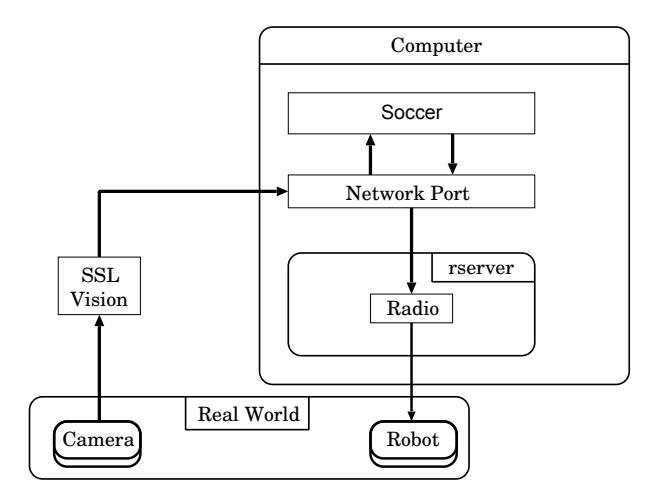
Figure 7 shows the overview of the RoboDragons system. The features of the system are as follows:
- Host computer is Athlon64 X2 4200+ with 512MB memory and Debian GNU/Linux OS.
- Each module(shown in box in Fig.7) is implemented as a thread.
- The Soccer module consists of a strategy, a tactics and a path generation submodules, and it produces an action command for each robot.
- Radio module sends the command to each robot through the radio system.
In the next sections, we describe the main improvements of our program.
3.2 Determining the number of mark robots
In our old strategy, the role of each teammate robot at the opponent free kick time was determined by the ball's position. For example, if the ball is within 500 mm from teammate goal line at the beginning of the free kick, it is considered to be an opponent corner kick and "3 mark robots" strategy is selected even if an opponent robot is out of field by a penalty. The program is improved to determine the number of mark robots dynamically as follows,
Let r^i be the position of the opponent robot i. If following conditions are satisfied, the robot i will be marked.
- – The distance between r^i and the center of teammate goal is less than R mm.
- – The distance between r^i and the teammate goal line is less than X mm, and there is a shoot course from r^i to the goal.
In RoboDragons, R = 3000 mm and X = 4600 mm. The number of mark robots ranges from 1 to 3.
3.3 Priority of mark robots
In RoboDragons, the number of teammate robots for marking is at most 3. However, there are cases that more than 3 robot should be marked at the opponent free kick. For example, the case four opponent robots are attacking. In this case, we select three opponent robots to mark. For each opponent robot, a priority is given as follows, and higher priority robots are selected.
– the greater the distance between r^i and the center of teammate goal, the higher the priority.
– the greater the affordance of the shoot course from r^i, the higher the priority.
There are two mark actions, i.e. pass cut mark and shot cut mark. The pass cut mark has two variations, i.e. preventing the pass at around the passing robot and around the receiving robot. The shot cut mark is as well.
3.4 Robots' actions at free kick
In the old strategy, teammate's pass action and shot action at free kick were as follows. In the following, we use the term "direct play" [2]. The direct play is one of cooperative plays, i.e. a passing robot kicks the ball to a recieving robot, and the recieving robot shoots the ball immeadiately when it gets the ball.
- – Pass action (passing robot in case of direct play)
- At time t0, the robot which has the greatest affordance of the shoot course is selected as a receiving robot of the pass.
- Passing robot moves to the waiting position Tr.
- When passing robot arrives at T^r at t1, it starts kicking action.
- After finishing the pass, passing robot waits there until the strategy change will happen.
- – Shot action (shooting robot in case of direct play)
- Search the best place to receive the ball and move there until the passing robot will pass.
- After passing, the shooting robot moves to the shooting position which is computed from the velosity of the ball and current self position.
- Shoot the ball. If shot is failed, then next action is taken.
New actions are,
- – Pass action (passing robot in case of direct play)
- At time t0, the robot which has the greatest affordance of the shoot course is selected as a receiving robot of the pass.
- Passing robot moves to the waiting position Tr.
- When passing robot arrives at T^r at t1, it starts kicking action.
- After finishing the pass, passing robot takes an attacker action.
- – Shot action (shooting robot in case of direct play)
- Search the best place within the specified region to receive the ball and move there until the passing robot will pass.
- After passing, the shooting robot moves to the shooting position which is computed from the velosity of the ball and current self position.
- If there are some candidates for shooting, the robot nearest to the teammate goal judges the possibility of shot. If it is not possible, then take a defending action.
In the RoboDragons 1-2-3 shot[2] using three robots, above shot action works well to reduce the time the goal keeper defends the goal without any other defender(s).
4 Realtime dominant region computation
(Section overview follows in subsections)
4.1 Need of realtime dominant region computation
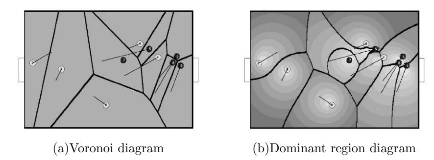
It is important to analyze the actions of opponent team in real time and then to change team's strategy dynamically in order to overcome the opponent, since the strategies based on them are growing year after year [3]. For such analysis, the voronoi diagram [4] and the dominant region diagram [5] are useful. They are used to analyze the sphere of influence. The voronoi diagram divides the region based on the distance between robots, while the dominant region diagram divides the region based on the arrival time of robots. It is considered that the dominant region diagram shows an adequate sphere of influence under the dynamically changing environment such as a soccer game.
In the SSL, the dominant region diagram has been used for arranging teammate robots to perform the cooperative play such as passing and shooting [2][6]. However, the existing algorithm takes much time to compute the dominant region diagram, the use of the algorithm is restricted to the case that the computation time can keep, i.e. a typical case is a restart of play. If the dominant region diagram can be computed in real time, we can apply it any time.
In this section, we describe the realtime computation of dominant region. In our system, it is required to compute the dominant region diagram within 5 msec. So, we put this time to be our present goal. Following algorithm is an approximate computation of the dominant region diagram so that we discuss the computation time and the approximation accuracy through the experiment. Our algorithm achieves 1/1000 times shorter in computing time compared with the algorithm proposed in literature [5] and over 90% accuracy. Moreover, 5 msec computation time can be possible under the parallel computers. We also show that the dominant region diagram is useful for the prediction of success for passing.
4.2 Computation of dominant region
A dominant region of an agent³ is defined as "a region where the agent can reach faster than any other agents". A dominant region diagram, simply a dominant region, shows the dominant region of every agent [5]. The dominant region diagram is one of the generalized voronoi diagrams. Though the dominant region diagram is an n dimensional diagram in general, we discuss a two dimensional diagram here because we consider a soccer field.
The dominant region is calculated as follows. Assume that an agent i is at the point $\mathbf{P}^i(=(P_x^i,P_y^i))$ and is moving at a velocity $\mathbf{v}^i(=(v_x^i,v_y^i))$ . Assume also that the agent can move to any direction and its maximum acceleration is $\mathbf{a}^i_{\theta}(=(a^i_{\theta x},a^i_{\theta y}))$ for a $\theta$ -direction. The position that the agent will be after t seconds is given by³,
$$\begin{pmatrix} x_{\theta}^i \ y_{\theta}^i \end{pmatrix} = \begin{pmatrix} \frac{1}{2} a_{\theta x}^i t^2 + v_x^i t + P_x^i \ \frac{1}{2} a_{\theta y}^i t^2 + v_y^i t + P_y^i \end{pmatrix}.$$
For given t, the set of above points makes a closed curve with respect to $\theta$ . Conversely, for given point $\mathbf{x} = (x, y)$ , we can compute the time which each agent takes⁴. Therefore, for each point $\mathbf{x}$ in a region (or a soccer field), we can get the dominant region by computing the following equation,
$$I_x = \underset{i}{\operatorname{argmin}} { t^i(\mathbf{x}) }, \tag{3}$$
where, $I_x$ is an agent's number which comes at first to the point $\mathbf{x}$ .
Preliminary experiment using the algorithm proposed in [5] shows that the computation time takes 10 to 40 seconds when the soccer field is digitized by $610\times420$ grid points.
³ We call a considering object (such as a player) an agent. ⁴ If more than one arrival time are obtained at point $\mathbf{x}$ for the agent i, the minimal arrival time is taken.
5 Approximate dominant region
To achieve a real-time computation of the dominant region, where the real time means a few milliseconds here, we propose an approximate dominant region. It can be obtained as a union of reachable polygonal regions. A reachable polygonal region is a polygon which is uniquely calculated when the motion model and time are given.
5.1 Motion model of robots
We define a motion model as a set of maximum acceleration vectors of a robot. Figure 9(a) shows an example of a motion model. Each maximum acceleration vector shows that the robot can move to that direction with the given maximum acceleration. This is an example of an omni-directional robot. Eight vectors are given. The number of vectors depends on the accuracy of obtaining the dominant region.
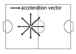
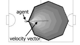
Fig. 9. Acceleration vectors and reachable polygonal region
5.2 Computation of reachable polygonal region
The reachable polygonal region is a region that is included in the polygon made by connecting the points, where each point is given as a point that an agent arrives at after t seconds when it moves toward the given direction of maximum acceleration vector in maximum acceleration. Eq. (2) is used to compute the point. Figure 9(b) shows an example of reachable polygonal region (shaded area) after 1 second passed when the acceleration vectors of figure 9(a) is given. We assume the reachable polygonal region is convex⁶. The reachable polygonal region is calculated by the following algorithm.
[Reachable polygonal region]
Step 1 Give a motion model of each agent (figure 9(a)).
Step 2 Give time t. Calculate each arrival point $(x_{\theta}^{i}, y_{\theta}^{i})$ according to the equation (2) using the corresponding maximum acceleration vector in Step1.
Step 3 Connect points calculated in Step2 (figure 9(b)).
⁶ If it is concave, we consider a convex hull of it.
5.3 Calculation of approximate dominant region
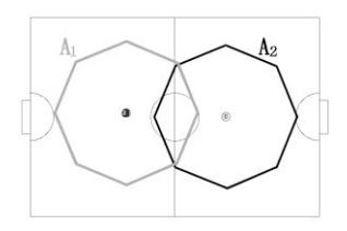
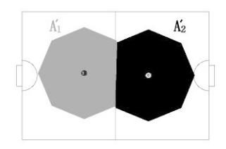
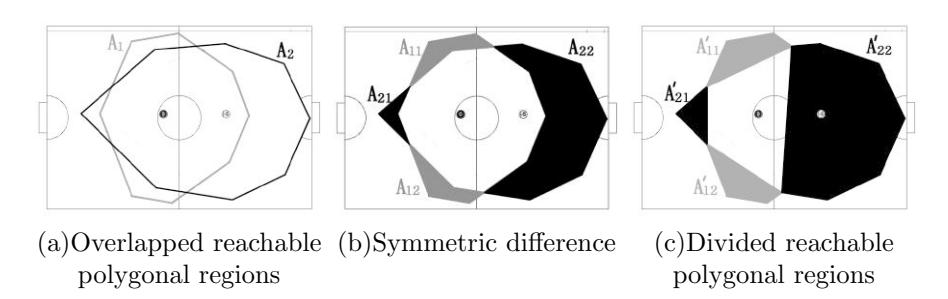
The approximate dominant region is obtained from the reachable polygonal regions for every agent. When some of reachable polygonal regions are overlapped, we have to decide which agent, the point belongs to the overlapped region. Figure 10(a) shows two overlapped reachable polygonal regions $(A_1,A_2)$ of two agents. In this case, it is natural to divide overlapped region into two by the line connecting the points of intersection of two polygons. Figure 10(b) shows a result for the reachable polygonal regions. However, since the number of points of intersection between two polygons (with n vertices) varies from 0 to 2n, we have to clarify the method of division for each case. Moreover, we need to consider the method of division when many reachable polygonal regions are overlapped. We describe these methods in the following algorithm. We call this an algorithm of the approximate dominant region.
[Approximate dominant region]
Step 1 For given time t, make a reachable polygonal region of each agent. (Figure 9(b)).
Step 2 For two reachable polygonal regions, if they are overlapped, divide the overlapped region in the following way. Generally, a number of points of intersection between two polygons with n vertices varies from 0 to 2n. If a vertex of one polygon is on the other polygon, move the vertex infinitesimally to the direction where the number of points of intersection does not increase. (There is no side effect with respect to this movement.) Therefore, the number of points of intersection is even. We show the way to divide in case of 0, 2 and 2k intersections.
- No points of intersection: There are two cases.
- (a) Disjoint: As two reachable polygonal regions are disjoint, there is no need to divide.
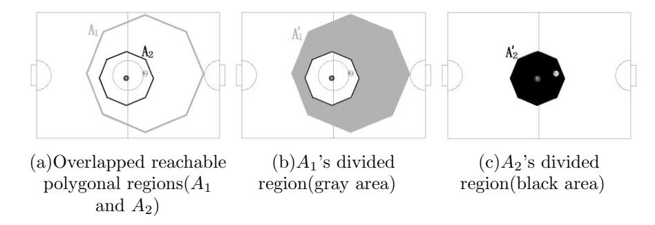
- (b) Properly included: One includes the other. Figure 11(a) shows an example $(A_1 \supset A_2)$ . In this case, $A_1 A_2$ is a dominant region of agent 1 (Fig. 11(b)) and $A_2$ is a dominant region in agent 2 (Fig. 11(c))⁷.
- 2 points of intersection: The overlapped regions of $A_1$ and $A_2$ is divided into two region by the line connecting the points of intersection between two polygons to create dominant regions $A'_1$ and $A'_2$ (Figure 10).
- 2k points of intersection: Let $A_1$ and $A_2$ be two reachable polygonal regions and I be a set of points of intersection between the polygons of $A_1$ and $A_2$ . Then, compute $A_1 A_2$ and $A_2 A_1$ . Figure 12(a) shows an example. In this example, there are 4 points of intersection. Figure 12(b) shows a difference between two regions, where $A_1 A_2 (= {A_{11}, A_{12}})$ is shaded in grey and $A_2 A_1 (= {A_{21}, A_{22}})$ is shaded in black. Make convex hulls of subregions. Figure 12(c) shows the result $(A'{11}, A'{12}, A'{21}, A'{22})$ . Thus, we have partial dominant regions $(A'1 = A'{11} \cup A'{12})$ and $A'2 = A'{21} \cup A'{22})$ of the agent 1 and 2. A white area in the overlapped region in figure 12(c) doesn't belong to either of two partial dominant regions.
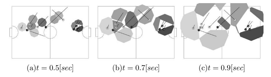
- Step 3 If n reachable polygonal regions $(A_1, A_2, \dots, A_n)$ are overlapped, we process as follows. First, for $A_1$ and $A_2$ , we take partial dominant regions $A'_1$ and $A'_2$ by using the procedure in step 2. Replace $A_1$ and $A_2$ with $A'_1$ and $A'_2$ . Then, for $A_1$ and $A_3$ , and $A_2$ and $A_3$ , do the same computation. Repeat this until $A_n$ is computed. As a result, we get new reachable polygonal regions $(A_1, A_2, \dots, A_n)$ where any two $A_i$ s are disjoint. These are the partial dominant regions of agents at given time t. Figure 13 shows three examples of partial dominant regions of 10 agents at time t = 0.5, 0.7 and 0.9 seconds.
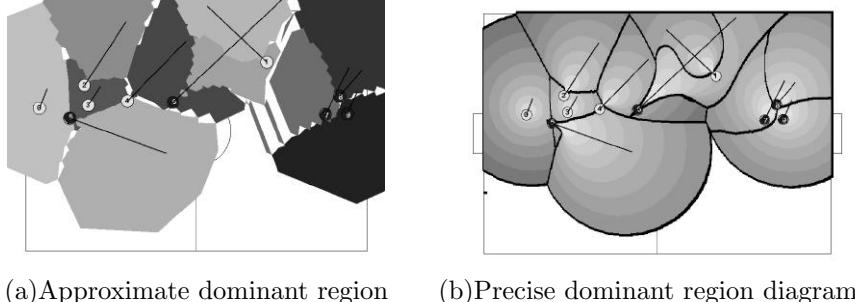
- Step 4 Synthesize the partial dominant regions incrementally. For given times $t_1, t_2, \dots, t_n$ $(t_1 < t_2 \dots < t_n)$ , compute the partial dominant regions. Let them be $B_1, B_2, \dots B_n$ . Then, compute $B_1 + (B_2 - B_1) + \dots + (B_n - \sum_{i=1}^{n-1} B_i)$ . This makes an approximate dominant region diagram. Figure 14(a) shows an example constructed from the examples shown in figure 13, but using 10 partial dominant regions computed by every 0.1 seconds.
⁷ This is not correct definition, but we adopt this to perform the real time computation.

6 Experimental evaluation for algorithm of approximate dominant region
(Section overview follows in subsections)
6.1 Experiment
In the SSL, since the ball moves very fast, the standard processing rate is 60 processings per second. One processing includes an image processing, a decision making, action planning, command sending and so on. Therefore, the allowed time for the computation of the dominant region is at most 5 milli-seconds⁸. Our purpose is to make the computation of the approximate dominant region within 5 msec.
⁸ This time constraint is sufficient when our algorithm will be applied for the other leagues in RoboCup soccer and human soccer.
Table 1. Computation time and accuracy of proposed algorithm
| acc. vectors | arrival-time steps | computation time [msec] | accuracy[%] |
|---|---|---|---|
| 8 | 10 | 17.5 | 91.8 |
| 8 | 20 | 33.8 | 92.9 |
| 16 | 10 | 31.4 | 95.3 |
| 64 | 200 | $2.4 \times 10^{3}$ | 99.9 |
| 2048 | 400 | $5.0 \times 10^{5}$ | 100 |
Table 2. Computation time on various computers (parameters: max acc. vectors: 8, arrival-time steps: 10)
| Г | CPU | proposed method(A) | existing method(B) | rate(B/A) |
|---|---|---|---|---|
| 1 | $3.16 \mathrm{GHz}$ | $17.5[\mathrm{msec}]$ | 13.3[sec] | 760 |
| 2 | 3.2GHz | $19.3[\mathrm{msec}]$ | 24.2[sec] | 1254 |
| 3 | 2.2GHz | 38.2[msec] | 40.5[sec] | 1060 |
| 4 | 2.2GHz | $38.3[\mathrm{msec}]$ | 40.4[sec] | 1055 |
6.2 Experimental result
We digitize the SSL's field into $610 \times 420$ grid points (1 grid represents the area of about 1 $cm^2$ ) and, for 10 agents (5 teammates and 5 opponents), compute the approximate dominant region that can arrive within 1 second. The reason why we set arrival time to 1 sec is that almost all of the whole field can be covered by the dominant region as shown in Fig. 14. We measure the computation time and the accuracy of the approximate dominant region. We define the accuracy by the following equation,
$$\text{Accuracy}[%] = \frac{\text{Total grid points that } I_x^d \text{ and } I_x^a \text{ coincide}}{\text{All grid points}} * 100 \tag{4}$$
where, $I_x^d$ and $I_x^a$ are given by Eq. (3) for the precise dominant region and the approximate dominant region, respectively.
We used the computer with Xeon X5460 as CPU, 8GB main memory and FreeBSD operating system for this experiment. We measured the computation time by running the program in a single thread.
The computation time and the accuracy of the approximate dominant region depend on the number of maximum acceleration vectors and the number of partial dominant regions (i.e. the number of time-divisions). We measured the computation time and the accuracy for the various values by using two parameters above. Figure 15 shows the results of the measure. Table 1 shows the computation time and the accuracy for some typical values of the parameters. The resulting approximate dominant region of the first row of the Table 1 is shown in Figure 14(a).
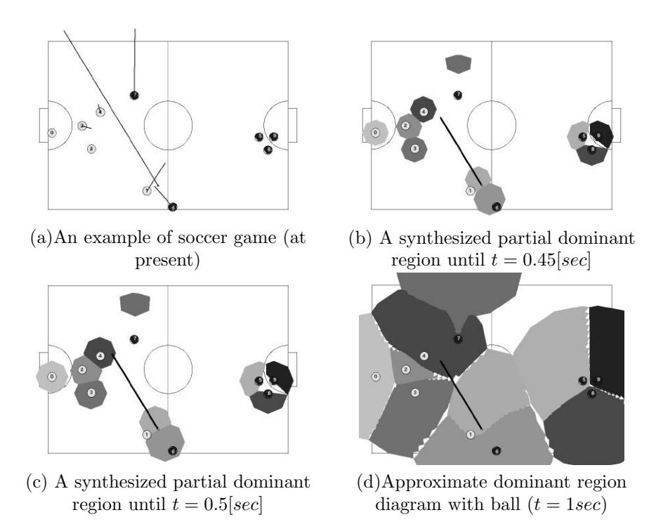
In comparison with Fig. 14(b), it is considered that Fig. 14(a) is a good approximation of the dominant region diagram. The accuracy is ranging from 91.8% to 100% from Table 1. These numbers show that our algorithm gives a good approximate dominant region.
Table 2 shows the computation time of the approximate dominant region diagram measured on the various computers. (The parameters on this experiment are fixed as the number of maximum acceleration vectors takes 8 and the number of time-divisions takes 10.) From the table, it is shown that the computation time can be reduced about 1/1000 times shorter compared with the algorithm shown in [5] and the accuracy keeps a little more over 90%. In addition, it is shown that, from Fig. 15(a), the computation time increases in proportion to the number of maximum acceleration vectors and the number of time-divisions, and from Fig. 15(b), the accuracy goes up rapidly to be 90% according to the increase of the number of maximum acceleration vectors and/or time-divisions, and then still slightly increases.
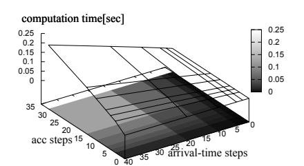
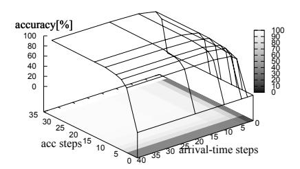
Fig. 15. Computation time and accuracy
6.3 Discussion
From Table 1, the approximate dominant region with parameters of 8 maximum acceleration vectors and 10 time-divisions achieves the accuracy of 92%. However, its computation time takes $17.5\ msec$ . It is a little bit far from our goal, which is computation time to be $5\ msec$ . To achieve this goal, we discuss a parallel computation here. Another issue whether the accuracy of 92% is enough in our purpose will be discussed in the next section.
In our algorithm, we create an approximate dominant region by synthesizing the partial dominant regions incrementally. Each partial dominant region can calculate independently and its computation time is almost equal for all the partial regions. The latter is supported by the fact that the computation time doubles when the partial dominant regions double. (See Fig. 15(a).) And also Table 3 shows an average time to compute a partial dominant region. For synthesis of 10 partial dominant regions, it takes 0.5msec on average. Therefore,
Table 3. Computation time necessary to make and to synthesize reachable polygonal regions
| acc. vectors | 8 | 16 | 24 | 32 |
|---|---|---|---|---|
| average computation time [msec] | 1.71 | 3.10 | 4.37 | 5.46 |
| standard deviation[msec] | 0.016 | 0.017 | 0.014 | 0.014 |
it is expected in parallel computation that the computation time will be about 1.71 + 0.5 + α msec when 10 partial dominant regions are synthesized, where α is an overhead of the parallel computation and is considered as a constant. In the multi-core parallel computer, the α is small enough. We consider that it is possible to make the computation time within 5 msec, which is our goal.
7 Prediction of success for passing
One application of the dominant region is the prediction of success for passing. In this section, we introduce a dominant region of a ball. The approximate dominant region takes a significant role to predict the success for passing. If we can predict the success of passing accurately in real time, we can choose a defense or an offense strategy appropriately.
7.1 Approximate dominant region of ball
We consider a dominant region of a ball. The motion of the kicked ball on the SSL's field can be considered as a uniform decelerated motion, since the ball receives the force by the friction of the field only, and the friction is constant over the field. In addition, the ball moves on a straight line unless it meets with an object. Thus, the dominant region of a ball is defined as a line segment that the ball does not meet with any agents. By using the following way, it is possible to find an agent who can get the ball first: 1) compute a partial dominant region for time t^i and draw the position of ball at time t^i on it. 2) If the ball is in the dominant region of an agent, then the agent can get the ball. if not, repeat computation for next time ti+1 until the ball is in the dominant region of an agent. By this way, we can predict the agent who gets the ball first, and also we can find a dominant region of a ball.
Figure 16 shows an example. Fig. 16 (a) is a current situation of the game. The ball is at the lower part of the left side from the center line. The lines in front of the agents and the ball show the velocity of them. Figs. 16 (b) and (c) are the synthesized partial dominant region until t = 0.45sec and t = 0.5sec, respectively. In Fig. 16 (b), there is no agent who can get the ball, but in Fig. 16 (c), the agent No. 4 can get the ball, since the ball is in the dominant region of the agent 4. Fig. 16 (d) shows the approximate dominant region until t = 1sec and the ball's dominant region. To make this diagram, it takes 0.5 msec more time than the computation time of the diagram without the ball.
7.2 Discussion
In this experiment, we use the approximate dominant region with parameters of 8 maximum acceleration vectors and 20 time-divisions for 1 second interval⁹. We used the logged data of the third-place match in 2007 RoboCup competition to analyze the prediction of success for passing. By using the proposed algorithm, we predict the robot who gets the ball first. 60 passings are predicted correctly out of 63 total passings in the game (95% accuracy), i.e. the predicted agent and the agent that gets the ball in the game coincide.
In the results, 3 passings are failed to predict correct agents. The detailed analysis shows that the cause of mis-prediction is not due to the accuracy of the approximate dominant region but due to the strategy of the team. That is, the mis-predicted agent acts to achieve an other goal like moving the goal area to defend the goal by the team's strategy instead of getting the ball. Therefore, we think the approximate dominant region is very useful to judge the prediction of success for passing as well as to evaluate the team's strategy.
⁹ It is possible to obtain the approximate dominant region within 5 msec under the parallel computation environment even if these parameter values are used.
8 Safety region
(Section overview follows in subsections)
8.1 Definition of safety region
A concept of "safety region" is simple. It is defined as a region that the teammate robot(s) can keep the goal when an opponent robot shoots the ball from the inside of the safety region if teammates are positioned properly according to their defence strategy. Remaining region of the field given by removing the safety region is called "unsafety region".
In the following discussion, as a first step, we do not consider the chip shot or the curved shot in the following discussion.
8.2 Calculation of safety region
The calculation of the safety region depends on how the shot action is taken, i.e. a single shot or a cooperative shot, and how the team keeps the goal, i.e. defence strategy and the number of defence robots. It takes much time to compute the precise safety region. Therefore, in the following, we describe procedures to compute the approximate safety region.
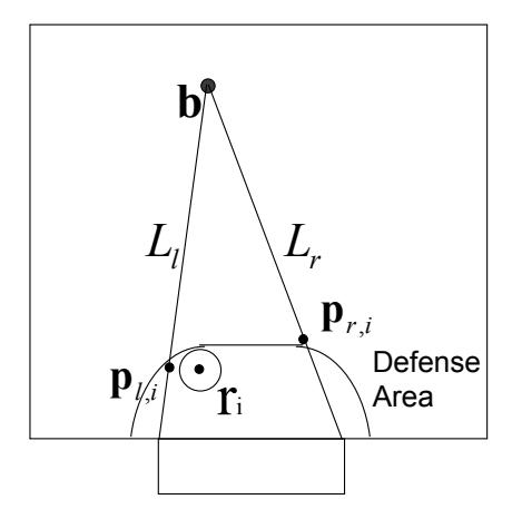
Calculation of approximate safety region: single shot case Defence robots will move according to their strategy so that we assume the right positions of the defence robots are given at any time. Let b be the position of the ball at time t. Let r^i be the position of the defence robot i at time t. Let L^r and L^l be the lines connecting b and the right and left goalposts, respectively. (See figure 1.) Defence robots usually stand on the inside of the region the lines L^r and L^l make. Let pr,i be the cross-point between the line L^r and the line perpendicular to L^r through r^i, and let pl,i be the cross-point similarly defined for the line L^l and r^i. Assuming *||r^i − pj,i|| ≥ R*, where || · || means a length of a vector ·, calculate the following equations for each defence robot i.
Compute,
$$t_s = \frac{||\mathbf{b} - \mathbf{p}_{j,i}||}{v_s}, \quad t_i = \frac{v_i}{a_i},\tag{5}$$
where t^s means the time for the ball to move from b to pj,i by the speed v^s and t^i the time for the speed of robot i to be v^i (starting from speed 0). v^i and a^i are the velocity and accerelation of the defence robot, and their values are decided depending on the defence strategy.
If t^i > ts, then compute whether equation
$$\frac{||\mathbf{b} - \mathbf{p}_{j,i}||}{v_s} > \sqrt{\frac{2(||\mathbf{r}i - \mathbf{p}{j,i}|| - R)}{a_i}}, \quad (j = r, l)$$
$$\tag{6}$$
is satisfied or not, otherwise compute whether equation
$$t_s > t_i + \frac{||\mathbf{r}i - \mathbf{p}{j,i}|| - R - \frac{a_i t_i^2}{2}}{v_i}, \quad (j = r, l).$$ (7)
is satisfied or not, where $v_s$ , $a_i$ , $v_i$ and R are the kicked speed of the ball, the maximal acceleration and velocity of the defence robot i, and the sum of radii of the defence robot and the ball, respectively.
When Equation (6) or (7) is satisfied for j = r and l, the position of the ball b is defined as a point in the safety region. In case there are more than one defence robot, if at least one of them satisfies Eq. (6) or (7), b is defined as a point in the safety region. When $||\mathbf{r}i - \mathbf{p}{j,i}|| < R$ is satisfied, b is also defined as a point in the safety region.
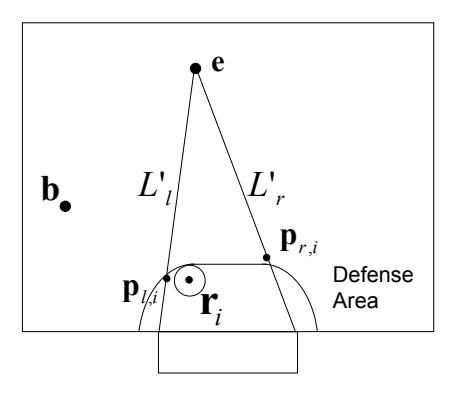
Calculation of approximate safety region: cooperative shot case When the two opponent robots make the shot cooperatively, a typical example is a direct play[2] which is an action that shooting robot kicks the ball immediately after receiving it from a passing robot (figure 2), we have to take the passing robot into consideration since the defence robots keep their goal at the positions that defend against the attack of both robots. In this case, we have to take the passing time into consideration to compute the safety region.
Let b and e be the positions of the ball and the shooting robot at time t, respectively, and $\mathbf{r}_i$ be the position of each defence robot i at time t. Let $L'_r$ and $L'l$ be the lines connecting e and the right goalpost and e and the left goalpost, respectively. (See figure 2.) We assume the goalkeeper stands in the defence area and moves along the defence area and other defence robots stand outside defence area and move along the defence area. Then, let $\mathbf{p}{r,i}$ be the cross-point between the line $L'_r$ and the line perpendicular to $L'_r$ through $\mathbf{r}i$ , and let $\mathbf{p}{l,i}$ be the crosspoint similarly defined for the line L' and $\mathbf{r}_i$ . Assuming that the passing robot holds the ball a obtained for cor
Compute,
$$t_p = \frac{||\mathbf{e} - \mathbf{b}||}{v_p}, \quad t_s = \frac{||\mathbf{p}_{j,i} - \mathbf{e}||}{v_s}, \quad t_i = \frac{v_i}{a_i}, \tag{8}$$
where $t_p$ means the passing time between b and e, $t_s$ and $t_i$ are the same ones in Eq. (5).
If $t_i > t_p + t_s$ , then compute whether equation
$$t_p + t_s > \sqrt{\frac{2(||\mathbf{p}_{j,i} - \mathbf{r}_i|| - R)}{a_i}}, \quad (j = r, l)$$ (9)
is satisfied or not, otherwise compute whether equation
$$t_p + t_s > t_i + \frac{||\mathbf{p}_{j,i} - \mathbf{r}_i|| - R - \frac{a_i t_i^2}{2}}{v_i}, \quad (j = r, l)$$ (10)
is satisfied or not, where, $v_p$ , $v_s$ , $v_i$ , $a_i$ and R are the speed of the ball at passing, the speed of the ball at shooting, the maximal velocity and acceleration of the defence robot i and the sum of radii of the defence robot and the ball, respectively.
If equation (9) or (10) is satisfied or there is no pass line¹⁰ between b and e, e is a point in the safety region. In case there are more than one defence robot, if at least one of them satisfies Eq. (9) or (10), e is a point in the safety region. When $||\mathbf{p}_{j,i} - \mathbf{r}_i|| < R$ , e is also a point in the safety region.
The length of the perpendicular from $\mathbf{r}_i$ to the line connecting $\mathbf{b}$ and $\mathbf{e}$ is less than the radius of the robot, it can block the pass.
¹⁰ The length of the perpendicular from $\mathbf{r}_i$ to the line connecting $\mathbf{b}$ and $\mathbf{e}$ is less than the radius of the robot, it can block the pass.
9 Experiment of safety region
(Section overview follows in subsections)
9.1 Method of experiment
The safety region should be calculated analytically, however, it is hard to do the analytic computation so that we calculate it on each of the mesh points which are given by dividing the field every 40 mm, and we give the approximate safety region using the model discussed in section 8.2.
On the other hand, to testify the correctness or preciseness of the proposed safety region, we compared the proposed safety region with the result of simulation, where simulation was done by using the game simulator embedded in the RoboDragons system. Here we show a simulation procedure for the cooperative play in the followings.
- Divide the field into n mesh points, where n = 14888 in this experiment. Put the ball on the initial position b, one of the mesh points. Also put the attacking robots on the mesh points, one around the ball and the other one a given point e^i, a shooting position¹¹. Place defence robot(s) on defending position(s) according to the strategy algorithm of the RoboDragons system.
- At time t, move the ball from b to e with the passing velocity vp.
- Move the ball on the shooting line from e which is the farthest line to the defence robots when the ball arrives at shooting position e at time te. (Shooting line is calculated at time t.)
- Simulate the movement of the defence robots and judge if a goal is achieved or not. If the goal is achieved, then the point e is a point in the unsafety region, otherwise it is a point in the safety region.
- Repeat steps 2 ... 4 for each point in the mesh by replacing e into it.
The initial position of the ball used in the simulation is selected from the logged data of the 8 games held in RoboCup Japan Open 2009 and RoboCup 2009, i.e. kick off, direct and indirect free kick points are the candidates of the initial position of the ball, and it is randomly selected from the candidates. Passing velocity and shooting velocity of the ball are 4.0 m/sec and 8.0 m/sec, respectively, which are the typical values in the SSL. The acceleration and velocity of the defence robot are 2.0 m/sec² and 0.6 m/sec, respectively, which are the measured values.
¹¹ We assume that the robot can kick the ball toward any direction.
9.2 Experimental results
Coincidence rate We compared the approximate safety region with the one obtained by the simulation for the one defence robot case and the two defence robots case under the RoboDragons's defense strategy. Figures 19 through 22 show the examples of the experimaental results.
In the figures, the white region is a safety region and the gray region is an unsafety region except the defense area in which the goalkeeper stands. There are two large gray areas in the field and the shapes of each area are similar between the proposed and simulated results. However, the down-left corner of the field does not match between the approximate results and the simulation results. (In the simulated result, there are many small gray dot-like areas. This is caused by the noise model implemented in the simulator.) These figures show that the approximate safety region is a well approximation of the safety region and can use as the safety region.
To show how much portion of safety and unsafety regions coincide with between the approximate method and the simulation, we define a coincidence rate R by the following equation.
$$R = \frac{\text{number of coincident points}}{\text{number of all points on the mesh}},$$ (11)
where coincident points are points that the results of approximate method and simulation coincide with. Table 4 shows the result which is the average of 10 trials.
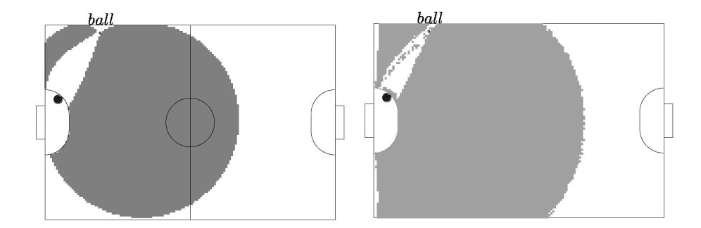
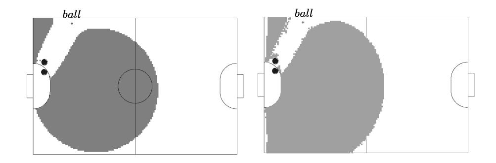
Table 4. Coincidence rate (Direct play[2])
| coincidence rate R | |
|---|---|
| one defence robot | 0.889 |
| two defence robots | 0.869 |
Computation time Using the three typical computers, we obtained the computation time for the proposed method. Table 5 shows the result.
In our system, given time for the computation of the safety region is at most 5 msec from our experience of the development of the RoboDragons system when we use the safety region in strategy computation in real time. From Table 5, we can realize the real time computation using the Xeon processor.
Table 5. Computation time
| CPU | Memory | one defence robot | two defence robots | |----|-----|----|----|----| | Pentium 4 2.8GHz | 1 GB | 4.5 msec | 5.6 msec | | Athron64 X2 4200+ | 512 MB | 4.6 msec | 6.1 msec | | Xeon 3.3 GHz | 2 GB | 1.5 msec | 1.9 msec |
10 A defence strategy using the safety region
(Section overview follows in subsections)
10.1 A defence algorithm using the safety region against the direct play
When n robots have already placed in defence positions and (n + 1)th robot is placed in defence position, the following algorithm determines the position of the (n + 1)th robot.
- Letting the positions of n defence robots be r^i (i = 1, ..., n), obtain the safety region and the unsaftey region. Number each connected component in the unsafety region. Let it be N^k (k = 1, ...)
- Search a connected component with maximal area (Nm) and compute the gravity center G of Nm.
- Place (n + 1)th robot at the cross-point of the line L^g and the defence line (a bit outside of defence area), where L^g is a bisector line of the maximal free angle toward the goal from point G.
Figures 23 and 24 are examples of the deployment of a new robot. Fig. 23 is obtained from Fig. 19 and Fig. 24 is obtained from Fig. 21. Figure 25 is the deployment of the three defence robots under the RoboDragons' existing strategy. Table 6 shows the number of points in the unsafety region.
From Table 6, it is shown that the proposed defence strategy (deployment algorithm) greatly reduces the area of the unsafety region. This means that it is possible to keep the goal to the great extent and shows that the proposed strategy is efficient against the opponent's cooperative play.
However, the proposed defence strategy is not always efficient against the opponent's cooperative play. For example, applying the proposed strategy to Figure 26, we get Figure 27.
In Fig. 27, if the shooting robot is in the unsafety region which is shown by the circle in Fig. 27, the goal is achieved by the robot. This situation is not preferable. In the next section, we discuss how we avoid such situation.
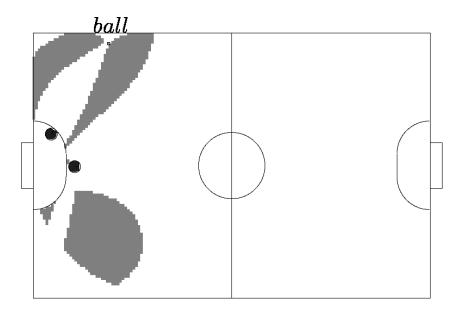
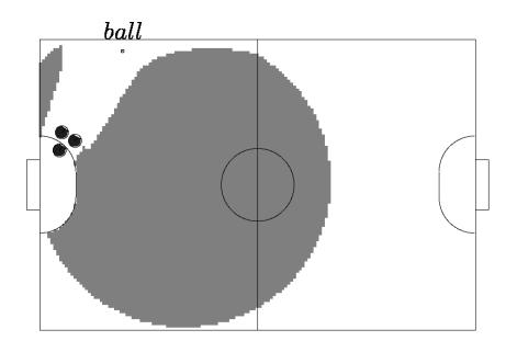
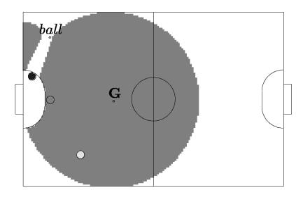
Table 6. the number of points in the unsafety region
| two defence robots | three defence robots | |
|---|---|---|
| existing strategy | 6256 (Fig. 21) | 7086 (Fig. 25) |
| proposed strategy | 1627 (Fig. 23) | 1126 (Fig. 24) |
Fig. 27. Safety region: two defence robots
10.2 A defence strategy considering the position of the opponent robot
In a real game, we should take the position of opponent robot into account. In this section, we discuss the weighted unsafety region. The weight is given to each point e in the unsafety region as a function of the distance between the position of the opponent robot r^e in the unsafety region and the point e. We gave the following weighting function,
$$w(\mathbf{e}) = \max(1, 100 \times (1 - \frac{||\mathbf{r}_e - \mathbf{e}||}{\max(M, t_p \times v_r)})). \tag{12}$$
In eq. (12), v^r is a velocity of opponent robot at r^e, and t^p is given by eq. (8). M is a threshold value to keep the weighting area wide when the value t^p × v^r is small. We used M = 270 in the experiment. w(e) takes the value in the range between 1 and 100.
Computing the weighted gravity center G′ of the unsafety region, and replacing G in the previous algorithm into G′, we get an improved algorithm for the placement of the defence robot.
Figure 28 shows a weighted unsafety region. The higher the weight, the darker the region. The weighted gravity center comes near the opponent robot in the unsafety region. Figure 29 shows obtained defence positions of the robots and an improved safety region. From the Fig. 29, it is clear that the opponent robot is in the outside of the unsafety region.
The computation time of the weighted gravity center and weighted (un)safety region¹² excluding the computation of weighted gravity center are given in Table 7. Comparing Tables 5 with 7, it is shown the increase of computation time by the weighted (un)safety region is small and the real time computation is possible.
¹² When stating computation time, we use the term "weighted (un)safety region", since it includes the computation time of both safety and weighted unsafety region.
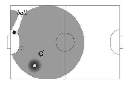
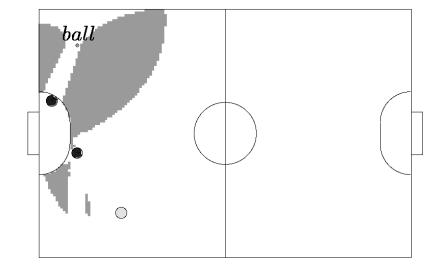
Table 7. Computation time of weighted (un)safety region
| CPU | Memory | Weighted gravity center | Weighted (un)safety region | |----|----|----|----|----| | Pentium4 2.8 GHz | 1 GB | 1.0 msec | 5.6 msec | | Athron64 X2 4200+ | 512 MB | 1.9 msec | 6.4 msec | | Xeon 3.3 GHz | 2 GB | 0.3 msec | 1.9 msec |
11 Concluding remarks
In this paper, we describe the configuration of the RoboDragons' new robots. The robot is driven by four DC brushless moters. A new control board is developed. There is not a large improvement in the software of the RoboDragons this year. A minar improvement is described. Research topics which will be embedded in the future RoboDragons system are described. The dominant region method and the safety region method. These can be used for realising a higher strategy.
acknowledgement
This work was supported by the cheif director's special study fund of Aichi Prefectural University and the president's special study fund of Aichi Prefectural University.
References
- "http://www.toppers.jp/en/index.html"
- Ryota Nakanishi, James Bruce, Kazuhito Murakami, Tadashi Naruse and Manuela Veloso, "Cooperative 3-Robot Passing and Shooting in the RoboCupSmall Size League", RoboCup 2006: Robot Soccer World Cup X, LNCS 4434 pp.418-425
- K. Murakami, S. Hibino, Y. Kodama, T. Iida, K. Kato and T. Naruse "Cooperative Soccer Play by Real Small-Size Robot", In RoboCup 2003: Robot Soccer World Cup VII, LNAI3020, pp. 410 - 421, Springer-Verlag, 2003
- F.P. Preparata and M.I. Shamos "Computational Geometry" Springer, 1988
- T. Taki and J. Hasegawa "Dominant Region: A Basic Feature for Group Motion Analysis and Its Application to Teamwork Evaluation in Soccer Games", Proc. SPIE Conference on Videometrics VI, Vol.3641, Pp.48-57 (Jan. 1999)
- R. Nakanishi, K. Murakami and T. Naruse "Dynamic Positioning Method Based on Dominant Region Diagram to Realize Successful Cooperative Play", In RoboCup 2007: Robot Soccer World Cup XI, LNAI5001, pp. 488 - 495, Springer-Verlag, 2007