MRL Extended Team Description 2011
Maziar Ahmad Sharbafi, Ali Azidehak, Mohammad Hoshyari, Omid Bakhshandeh Babarsad, Aras Adhami-Mirhosseini, Alireza Zareian, Danial Esmaeely, Amin Ganjali, Saeed Esmaeelpourfard, Sajjad Ziadloo, Hamidreza Jamaati Tafti
Islamic Azad University of Qazvin; Electrical Engineering and Computer Science Department; Mechatronics Research Lab; Qazvin, Iran
Abstract Small size soccer environment, did not change significantly in the shape and challenges for about three years. With this attitude, it seems that some teams like Skuba have reached nearly the best achievable performance and other teams try to approach them. Producing reliable hardware architecture is the first step and improvement of the control and strategies are the following ones. MRL small size soccer team with more than three years experience in different international competitions is planning to complete all requirements to reach such goals when participates in 2011 world games. After attaining acceptable performance to reach the third place in 2010 competitions, debugging, increasing the reliability and achieving higher accuracy and speed are the next steps in our modifications for this year. Finalizing our debugging tools like 3D simulator and comprehensive user interface in this year aided us to evaluate whole of the system software from low level control to high level strategies. Also, redesigning the electronic boards and mechanical structure promoted the robot abilities in performing more complicated tasks. In Iran open 2011, desired speed beside acceptable accuracy in motion control was satisfied and it is observed that some parts of mechanical designs need some modifications. Finally, it is concluded that in spite of our high quality high level in robot intelligence, minor problems in control and debugging processes are still existed.
1 Introduction
MRL team started working on small size robot From 2008 and after three years we could qualified to be in semi final round and attaining the third place which means that our last year plan was achieved. The main problem in MRL robot in 2010 competitions was its unreliable behavior. Our main target in this year plan is resolving this problem via redesigning the electrical and mechanical mechanisms.
Another goal of our team is improving the speed and accuracy of the motion. Some requirements to reach this target are satisfied with hardware restructuring. New methods in control are designed using abilities gained by evolution of software tools like online debugging tools and simulator which is detailed more in [2]. Iran open 2011 was an opportunity to evaluate our new contributions. Although, our hardware was prepared too late, the results are noteworthy for us. Shortage of time avoids us
from finalizing our designs completely, but it is promising to have appropriate quality in the future. Being the first team in these competitions' technical challenge shows our hopefully progress even better than the best team of SSL competitions in recent two years (Skuba).
This paper is organized as follows: Firstly, software architecture including our new approaches in high level strategies and tools are described in section 2. A new electrical design based on Arm micro controller beside FPGA, and other accessories of robots' onboard brain, is explained in section 3. Description of mechanical configuration modification for the newly designed robot which elevates the capabilities of the robots' smooth and reliable motion is the subject of section 4. Finally, our new contributions about motion control which has a key role in robot performance is the subject of the last section. Further research on this topic to reach the perfect motion control is under investigation too.
2 Software
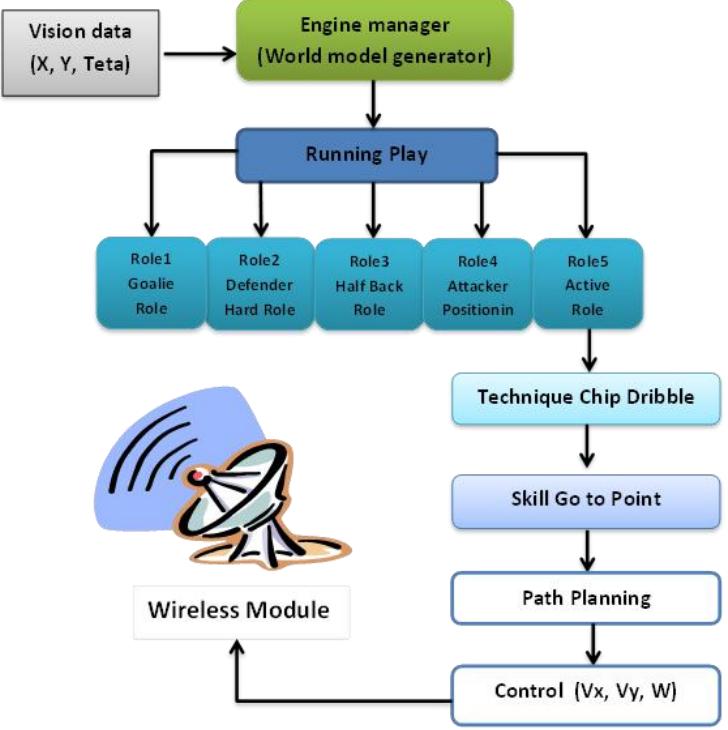
In this part the software main objects are presented. It is shown that how our new system debugger helps us to design a robust controller and microprocessor programs. In this year MRL software team has been started a new high level analyser project that will be shown in the next section. Our simulator's new features will be presented afterward. Our game plan contains many parts like roles, techniques and skills. Fig. 1 displays the relations between different parts. In this diagram, an instance of a play with its hierarchy to manage other required modules are depicted. Explanations about these objects are explained in our previous TDPs [3]. In this paper concentration on a new layer, named technique, is explained in the following.
Our method for kicking incoming pass in a specific point and some points about reinforcement learning which is utilized in passing mechanism are the remained parts of this section.
2.1. Techniques
Techniques are a new layer that has been added to our software architecture. Techniques have been placed between Role's layer and skill's layer. Skills like "Goto-point" or "Rotate-to-point" are simple skills which are used in techniques. The attacker robot does some movement to change the conditions for performing its selected techniques. Each technique has a cost function that shows its feasibility to be executed. Always the technique with minimum cost and maximum feasibility has been selected. Each permitted technique can be chosen based on its priority parameter. There are three main movement strategies about our game, moving to opponent goal, moving horizontal or vertical. Techniques have to perform their movement with all three main movement strategies. With choosing the main movement strategy, techniques help us to move the ball totally to the desirable target. Some of the techniques are introduced in upcoming subsections.
2.1.1 Aim and Kick Technique
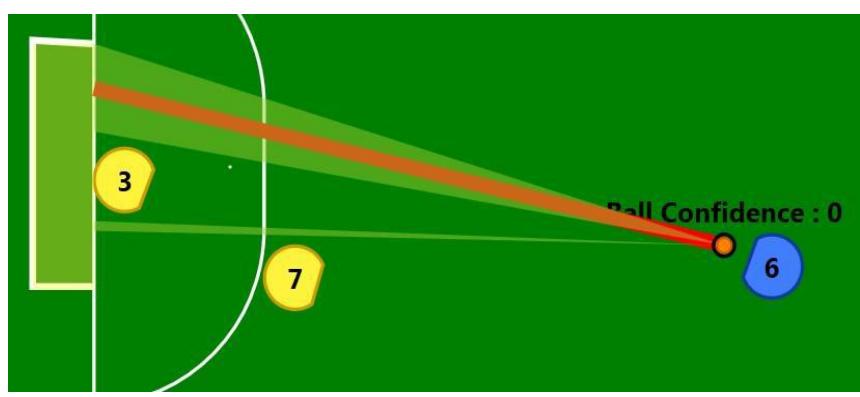
The "aim and kick technique" which usually has the highest priority is responsible for preparing the robot to kick the ball to the opponent's goal in the case of feasibility of scoring the goal. Firstly, we should recognize the best empty space in the opponent's goal. This space is not always the largest one and we should also consider other points like robot's movement direction, blocking robots' angels and velocities. Fig. 2. shows an instance of detecting the best opening area of the goal.
2.1.2 Space Dribble Technique
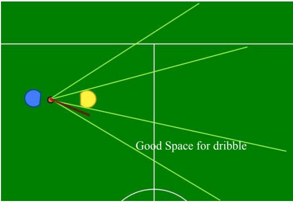
"Space dribble" technique is devised for dribbling the ball straight forward with leading the ball in the case of having adequate space. Also this technique is created for possessing the ball by moving towards it and in this way 50cm ball carrying constraint is prohibited too. First of all it should be assessed whether the robot has enough space for its intended movement or not. For this issue each robot should consider congestion of all other robots in different adjacent regions of the field. After that, the best place is selected among all candidate spaces. Note that it is possible to select none of them which means that the technique is not efficient. In our approach, to avoid the risk of giving opportunity to the opponent, space dribble technique is executable when the robot possesses the ball in the middle of the field.
2.1.3 Chip Dribble Technique
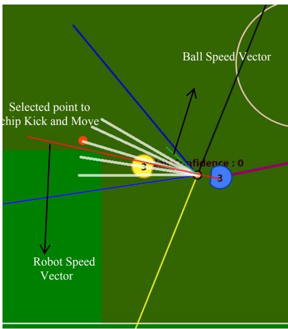
"Chip dribble" technique is another kind of dribbling to pass the blocking opponent away using a short chip kick. This technique is prone to loss of the ball so that it has the lowest priority. Criteria such as opponent robots congestion right behind this robot, movement direction of opponent robots and ball owner's movement angel are considered for ranking this technique. In the case of feasibility, one location behind opponent robot is selected in order to chip kick the ball to the designated location. The robot should move to that location promptly which will surprise opponent robot. The algorithm for calculating this location is as follows: hypothetical lines connecting ball to the opponent robot are drawn. The ending point of each line is considered and the best one is the point that has proper distance from opponent robot. This technique is applicable in the case of having 25cm distance from the opponent robot in order to be able to shoot the ball over the opponent in the air. Also, in order to decrease the risks we don't apply this technique in our own half field.
2.2. Online internal debugging
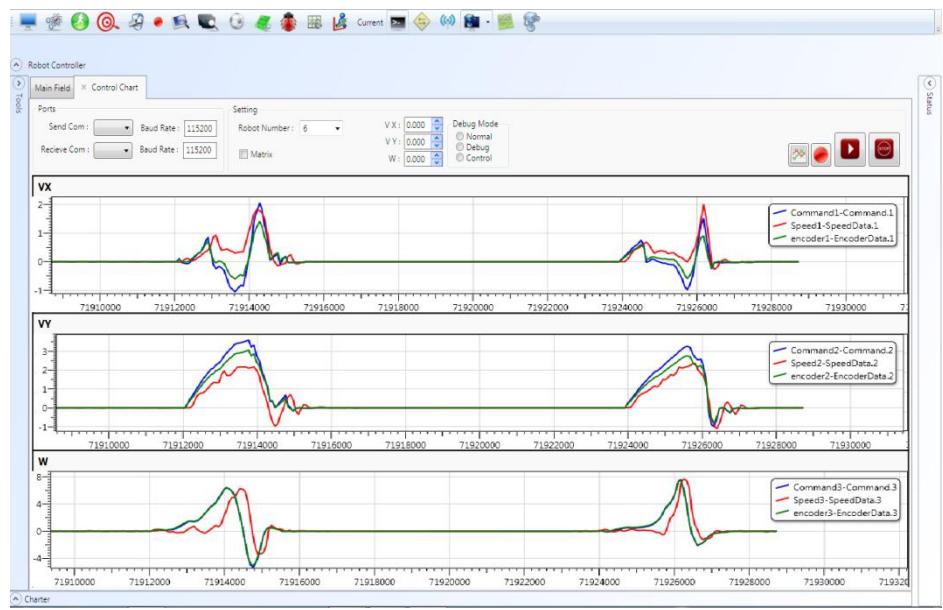
As stated before, to debug onboard control modules such as wheels' speed and controller parameters a comprehensive debugging tool is required. Simultaneous investigation of the commanded and the robot velocities (computed via vision and encoder data) is desired. Using this new approach we can easily debug and analyze our PID controller, wireless module data or any of our internal components. We've designed an online link between our microprocessor and AI systems in order to debug and maintain all controllers and speed problems easily and in a time optimal fashion. Fig. 5. shows our internal debugger graphical interface. If the desired velocity and the robot speed measured by vision are similar, the control performance will be suitable.
Previously, we had a unique configuration states for all of the robots without considering differences between them. This year, we have embedded a sub-section to our AI system which stores specific properties of each robot which later would be used for system's calibrations. These properties include controlling issues, kick speed or any kind of configuration parameters.
2.3. Applying Reinforcement Learning
Temporal Difference learning, first introduced by Samuel [4] and later extended and formalized by Sutton [5] in his TD() algorithm, is an elegant technique for approximating the expected long term future cost (or cost-to-go) of a stochastic dynamical system as a function of the current state. The mapping from states to future cost is implemented by a parameterized function approximator such as a neural network. The parameters are updated online after each state transition, or possibly in batch updates after several state transitions. The goal of the algorithm is to improve the cost estimations as the number of the observed state transitions and the associated costs increments. We find out that this elegant technique could be useful during online dynamic game. The pseudo code of TD is illustrated in Fig.6.
Initialize V(s) arbitrarily,  to the policy to be evaluated
Repeat (for each episode):
      Initialize s
      Repeat (for each step of episode):
               a ← action given by  for s
               Take action a, observe reward, r, and next state, s'
               V(s) ← V(s) +  [ r +  V(s') - V(s) ]
               s ← s'
      until s is terminal
Fig. 6. Tabular TD(0) for estimating V
Therefore, one can benefit from this robust method in low and high level of decision making e.g. in making decision about direction of kick in non-static balls. When the robot pass the ball to another one, the speed of moving ball in the vicinity of the second robot interferes in the direction of final kick to the target. To control this problem, Temporal Difference could be applied.
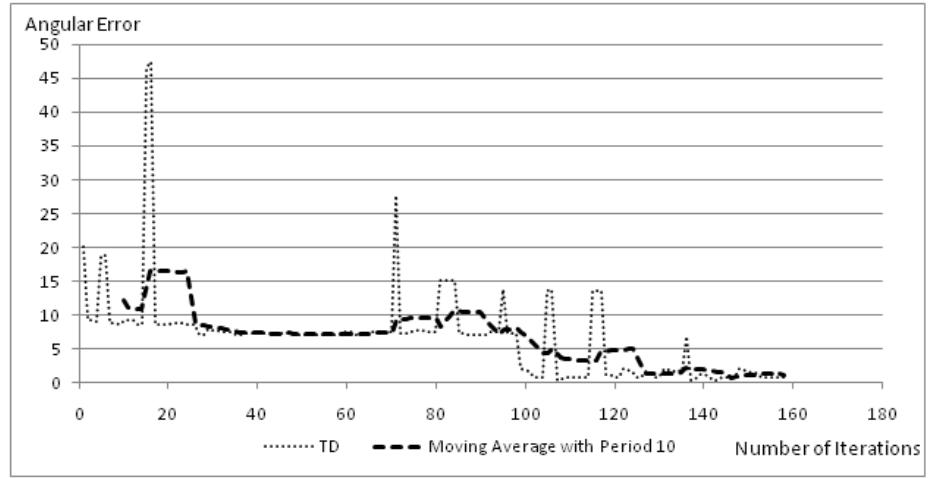
Rewards of kicks in the vicinity of the target are calculated and learning loop is triggered after each kick. To evaluate the method performance, at first it was tested on our 3D simulator. The results of this reinforcement learning approach show that after several runs, the correct direction will be determined (see Fig. 7).
Another technique which can be useful in decision making is Q-Learning. Many problems can be modeled as a discrete markov chain and Q-Learning addressed as a proper method to overcome these difficulties. After calculating Q-Value the best path to achieve the goal is obtained. For example, suppose 2 defenders aren't fast and after 2 passes they would be confused. So, Q-Learning shows a path between many states that contain a lot of passes from side to side to make opponents dizzy and last state is a kick. Fig. 8 depicts the algorithm of Q-Learning. In Iran open 2011 we evaluated our learning in technical challenge (passing stage) which had surprising results.
In [6] we have utilized some other learning methods like emotional learning for robot motion control. Such fast learning approaches are in our future viewpoint for learning different tasks too.
2.2. High level Analyzer
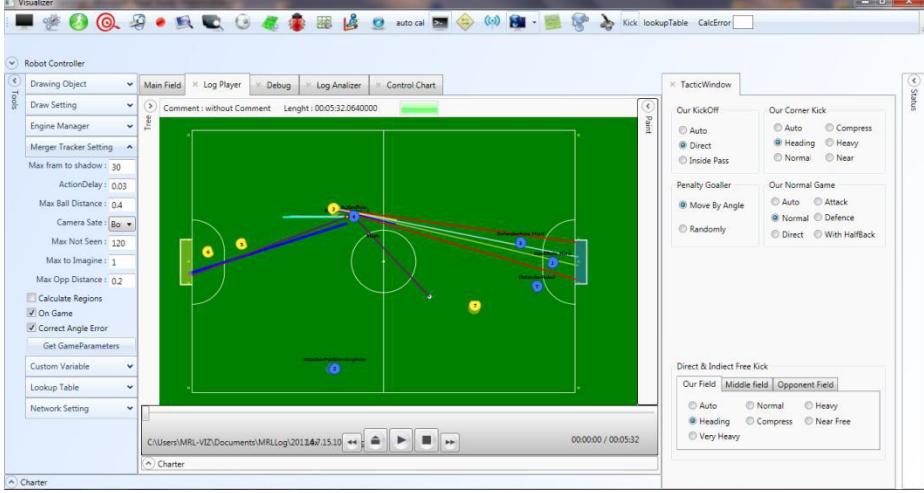
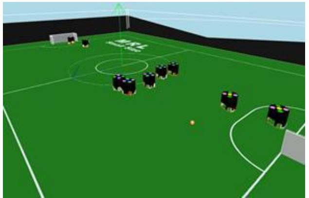
One of the most significant variations we have made to our MRL2011 team is the implementation of a new decision making layer as a high-level analyser (Fig. 9). Log files from SSL Vision of all MRL games should be recorded during a game. The final stage is the extraction of the opponent team strategies and finding the best tactic to cope with it. Although, it is too far from implementation, the preliminary steps are under construction. Strategy model consists of different parameters such as the number of robots in each position e.g. defence robots, attackers and free robots. Our goal is distinguishing the best feasible strategy from these models dynamically. For instance, if the opponent team is attacking with one "attacker", one marker robot should be placed to block it. If there are two attackers in non dangerous area (far from penalty area), there should be still one blocker robot. Of course, such high level decision makings can be implemented properly when each task in lower levels could be performed in a perfect manner. Before obtaining such performances a simulator will help the high level designer to evaluate his ideas (fig. 10).
The core system of MRL2011's simulator is the same as MRL2010. One of the significant changes in the simulator is considering noise signals in wireless system. We found that this noise has a close relation with distance. Sometimes data packets aren't properly received by robots. A probabilistic model for data transfer has been introduced to simulate a real wireless system. Measuring lost data compared with the size of sent packets shows a detectable relation with distance between the robot and the wireless transmitter (d). A Gaussian distribution is fitted to the wireless noise with the mean (m) and variance ( related to the distance ((1) and (2)). More details about these contributions are explained in [2].
$$m = (1 + \frac{2}{\pi}\arctan(0.4(d-5))) \tag{1}$$
$$\sigma = 0.03\log(1 + \frac{d}{5})\tag{2}$$
Because of latency in finalizing the robot hardware structure, investigation of the codes from high level strategies to each skill performance need an environment similar to the reality. Fortunately, progressing of the simulator prepared such an environment and our tests in simulator not only specified our bugs but also give some new points about implementation on real robots. Besides these preferences, this mechanism prevents the robots from damaging. As stated before, our learning algorithms after evaluating on the simulator made an appropriate basin to converge in real world.
Another point is about the analyzer which simplifies our operations as much as possible. From availability of changing the game strategy to demonstration of the game status and drawing the diagrams and necessary shapes to analyze the game conditions and detect the mistakes are achievable with this tool. In near future we will complete the entire requirements to play with a team of the robots with a virtual team in the simulator that satisfy our need to have friendly matches.
3 Electrical Design
In this section, different parts of electronic boards will be investigated. The robot has a main board and different module boards connected to it. It includes, Processor Daughter Board (PDB), motor driver modules and solenoid driver circuit. A wireless board is also designed to send and receive data between robots and AI system. In the following these concepts are described in detail.
3.1. Main Board
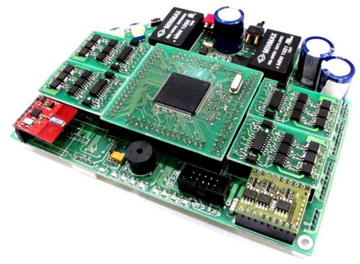
Current main board is the product of 4 years designing and evaluating. Last years, we've got problems with different circuits, causing damages and extra maintenance. Hence, we decided to add more protection circuits and improve our designs. Fig. 11 shows the main board of the robot.
Main problems of these boards which are related to the main board can be sorted as follows:
1. Charger Board:
- Charger board keeps 250V in capacitors. Any failure in this circuit cause harmful damages in the robot.
- Because of the weak insulation between solenoid and mechanical structure, a spark can happen between them at the kicking time.
2. Motor Driver:
- There were lots of damages in MOSFETs, fuses and current resistors because of high starting current in the motors.
- Since the input of MOSFET driver is connected directly to the PDB pins, any failure in motor driver might affect that module.
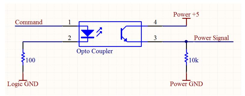
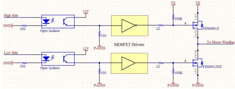
All of these problems are the results of connecting whole circuits together with same ground plane. For decreasing such problems, the separation of power and logic sections was chosen. To transfer signals between these sections, commercial low speed optocouplers (PS2801) were used. In figure 12, schematic of using these devices is illustrated.
Isolation of signals doesn't necessarily assure that power section won't affect the logic section. Whenever current flows in power devices, electrical potential of supply nodes will change and this effect can destabilize the power supply circuit. In order to eliminate this effect, both ground nodes must be separated. Hence, a DC/DC convertor with internal transformer was chosen as a an appropriate solution to isolate both sections from each other.
3.2. Processor Daughter Board (PDB)
Two years ago, we utilized Altera™ FPGA for our all electronics' purposes such as control, driving and so on. Although real-time advantages of FPGA are so useful, we suffered from some limitations. The first one was debugging, since there was not any reliable and user friendly method for detecting system errors. Due to the soft core emulation implemented in FPGA, the interrupts did not have enough speed which was the second problem. Moreover we used an external memory for storing data. From this point of view that the external memory is considered as an I/O device, data transmission does not have appropriate speed.
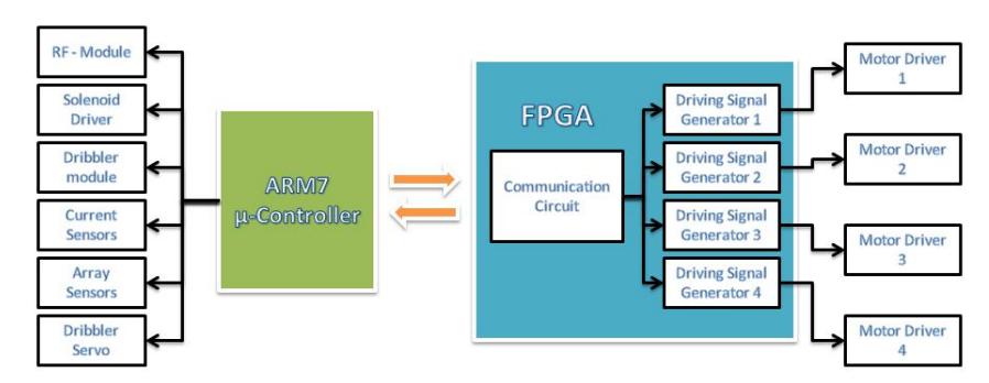
Because of the drawbacks mentioned above, we decided to utilize ARM7 microcontroller beside FPGA. It was selected for several reasons such as its powerful debugging capabilities and low-power design of ARM architecture. In addition, the ARM7 with TDMI-S core is one of the best choices for system control. Hence, only real-time tasks such as motor driving are executed in FPGA and all remained parts are implemented in ARM7 microcontroller. Figure 13 represents the relation between ARM and FPGA. According to this figure, the FPGA sends the encoder data and in other side, the ARM microcontroller prepares PWM data for FPGA to drive the motors.
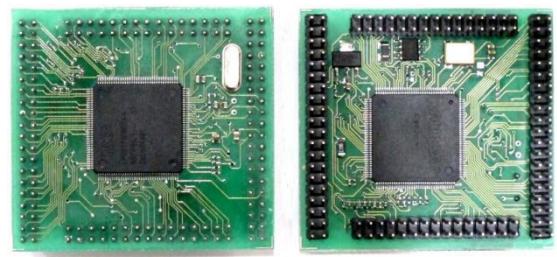
The PDB consists of one FPGA (Altera™ Cyclone® - EP1C6T144C8) and one ARM processor (NXP™ – LPC2378) connected to each other. FPGA duty is to control the motors and ARM processor is used to control the FPGA, communicate to wireless, compute control algorithms, debug the entire system and log the data. We used ARM7-TDMI core and developed the project in KEIL™ software. Figure 14 represents the up and down views of the PDB.
Our ARM7 microprocessor software architecture is designed by two main interrupts:
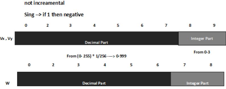
- 1- Wireless Interrupts: This event occurs when a new packet is received by our nrf24L01. The frequency of this event is about 60 HZ which is sent by AI console and the size of packet is 32 bytes. Our packets kind is classified in three main categories. The first packet kind indicates motion data and the second one contains our tuning parameters like controller parameters. Last packet kind is used for the wireless channel properties. When this packet is received by the wireless module, the microprocessor changes the nrf24L01 working channel and restarts it by new parameters. The online game movement packet has been shown in fig.15.
- 2- Control Interrupt: This interrupt occurs each 2 milliseconds. Every two milliseconds a PI control function runs for each wheel which gets its desired speed from wireless packet and its feedback speed from FPGA.
Also some interrupts like ADC protection interrupt are placed in our microprocessor software architecture. The ability of our software is online debugging from serial interface that is utilized for tuning controller parameters. Also we can test and configure different parts of the robot from configuration interface which is designed by some switches on the main board. For example we can set robot ID and wireless channel and test motors, kicker and spin back by this interface.
3.3. Batteries and protection
Each robot is running on two pack of Li-Polymer (Dualsky™ – xp21002ex) batteries with total voltages of 14.8 volts and capacity of 2100 mAh. These kinds of batteries are very sensitive to overuse. If the voltage of each cell is dropped below 3 volts, the cell would be damaged permanently. Hence, a battery protection circuit and a low voltage alarm (buzzer) are used. This circuit turns the system off when voltage of each pack is dropped below 6.8 volts and the alarm goes on when the voltages dropped below 7 volts. It also sends the voltage value back to the AI system to be monitored.
3.4. Wireless communication
The communication between robots and AI system is done by using two nRF2401 transceivers. These modules work in frequency between 2.4 to 2.525 GHz. Designing printed circuit board (PCB) of RF circuits needs special skills and facilities, so the ready to use module (sparkfun™ – WRL00691) was used.
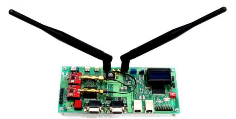
A wireless board (Figure 16) was also designed to ease the process of sending and receiving packets from modules to AI system. Since changing each module from the receive mode to the send mode consume some time, two separate modules are employed to decrease this delay. The output power of nRF2401 chip is limited to 0 dbm, so a radio amplifier (BBA-519-A) is used to increase the output power up to 18 dbm (50 mW).
The environment of Robocup competition has lots of interferences caused by different teams. An intelligent algorithm was used to scan different frequency channels and calculate data loss in each one. After that, the best frequency will be used as working frequency.
3.5. Charger
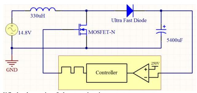
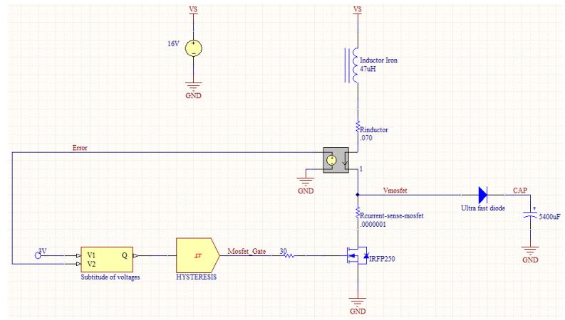
The system of charger in the robot is combined of solenoids, capacitors with high voltages and MOSFET switching circuit. The robot runs with supply voltages of 14.8V. In order to have powerful kicks, high magnetic field is needed and this can be gained by flowing high current in the solenoid. Since the solenoid has internal resistance, a high voltage is needed. There are different circuits that convert a voltage to higher values including voltage multiplier circuit, boost converter and etc. By evaluating different circuits, boost converter was finally chosen. The simplified circuit of the charger is shown in Fig. 17.
The process of conversion can be divided into two periods (Fig. 18). When the power switch (IRFP460) is on, energy is being stored in the inductor (330uH). After turning the switch off, the inductor transfers its electromagnetic energy to the capacitor (5400 uF – 250V), by turning the diode on. The equation of these energy conversions are stated in (3)-(7). By repeating this cycle, capacitor voltage would increase in several seconds. This Voltage will be used as the power supply for kickers.
$$E_{Inductor} = \frac{1}{2}LI^2 \tag{3}$$
$$E_{1Capacitor} = \frac{1}{2}CV^2 \tag{4}$$
$$E_{2Capacitor} = \frac{1}{2}C(V + \Delta V)^2 \tag{5}$$
$$E_{2Capacitor} - E_{1Capacitor} = CV\Delta V = \frac{1}{2}LI^2$$ (6)
Therefore:
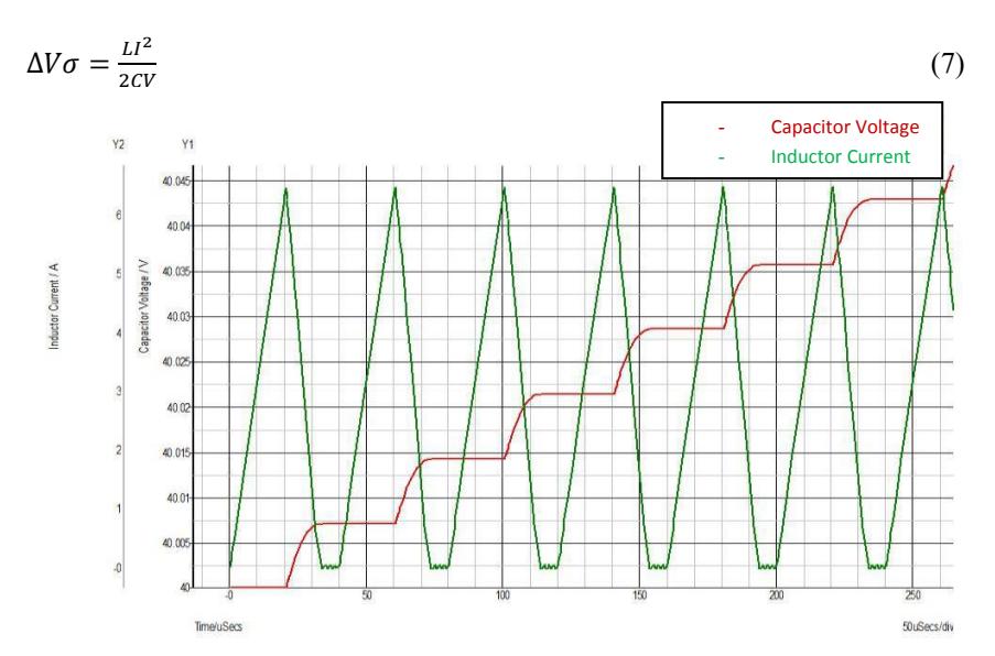
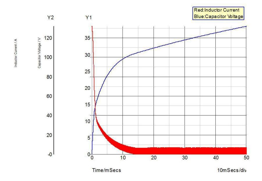
The important parameters in designing switching circuits are the frequency and the pulse width of the driving signal in power switch. There is a tradeoff between the charging time and the power consumption. The drive signal must be set in the way that assures the inductor won't enter the saturation region. The inductor acts as a resistor in this region and consumes the energy in its body. In practice, the 5 KHz frequency with duty cycle of 75 percent for 330uH inductor is chosen for the charger circuit. Although it is simple to have constant driving signal, it is not the optimum solution. As shown in figure 19, the inductor's current would be so high that it works in saturation region at the starting time.
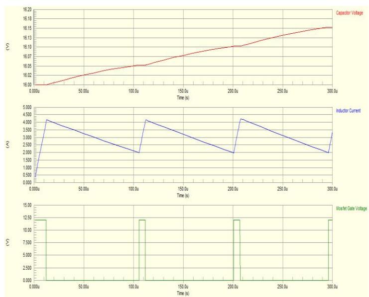
To avoid this problem and not having dead time after storing inductor energy in the capacitor, hysteresis mode can be used. In this method, an upper threshold point (UTP) and a lower threshold point (LTP) are set for the inductor current. If the current goes higher than UTP, power switch will be turned off and if it goes below the LTP, it will be turn on again. As figure 20 shows, inductor current will swing between two points and it won't go to saturation region.
This method was tested in practice (figure 21), but because of the space limitation, the old model is still used in the robot.
3.6. Kicker
The kicker system in robot is working based on the force created by a ferromagnetic plunger in the coil of the solenoid. Force created in the solenoid is depended on several factors, including number of turns in the coil, material of the plunger, its weight, the value of the current in the coil, duration of switching of power MOSFET and extra mechanical factors.
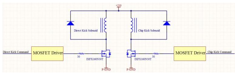
There are two separate kicker systems in the robot. One cylindrical type is used for direct kicks and another flat type is used for chip kicks. Therefore, two separate MOSFETs were used to flow current in solenoids when it is needed. The circuit for driving solenoids is presented in Fig 22.
Designing solenoid needs noticeable knowledge and experience in the field of electromagnetic analysis. The team members used experiences of other teams and did experimental tests with considering the basic concept of the electromagnetic field. Finally by considering space limitations, a cylindrical solenoid with 6 layers of 0.7 mm wire (70 rounds in each layer) is used for direct kick and a flat solenoid with 5 layers of 0.6 mm wire (50 rounds in each layer) is used for chip kick.
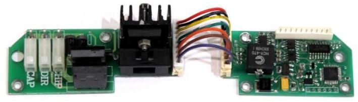
Charger and Kicker are separated from the main board. They are installed on the mechanical structure, apart from the main board. Figure 23 shows both charger and kicker boards, connected to each other.
3.7. Motor
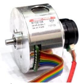
The robot has 4 Brushless DC Motors (BLDC) to perform precise motions. BLDC motors are MAXON™ flat motor (EC45 - 50 watts) with custom back extended shaft combined by US Digital™ E4P encoder with 360 counts per revolution which is 1440 pulse per revolution (Figure 24). In dribbler module, a MAXON™ EC16 - 50 watts motor is used as an actuator. To drive this motor, ready to use module (DEC module 24/2) is used.
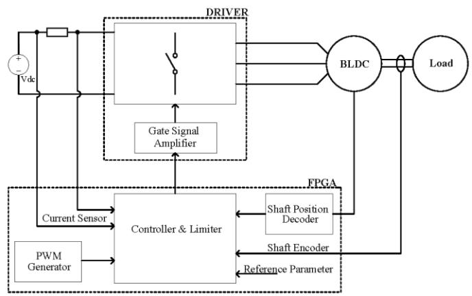
To drive this motor, internal hall sensors are used. According to the current status of hall sensors, driving signals would be created for power MOSFETs. This operation is being done in FPGA located in PDB. As displayed in figure 25 , the driver circuit in the FPGA, get samples from motor current, hall sensor status and rotary encoder connected to the motor to perform control tasks [1].
Created signals should turn the power MOSFETs on, but their levels at FPGA pins are not sufficient to do that. Hence, MOSFET driver would be used to amplify these signals. Last years, power and logic sections have a unique ground plane, but this year, these sections are separated as discussed in previous sections. To transfer signals between two sections, optocouplers are used. The total delay of 4 micro seconds from input to output of optocouplers is gained, which is high in switching circuits. A protection circuit was implemented in FPGA that considers a delay of several micro seconds between each transition of output signals to assure that low side and high side power MOSFETs won't turn on simultaneously. Figure 26 demonstrates the schematic of one stage of motor drivers.
Motor driver has internal current limitation for protecting motor from damages, but this method is not accurate for control applications. In order to increase the precision in sampling of the motor current, hall-effect current sensors (ACS712) are utilized. An ingenious algorithm was implemented to decrease the PWM of motors when they exceed the threshold specified by the controller module. This action can decrease slips of the wheels in playing field too. These sensors also help us to find out the problems of motors, especially when driver module doesn't work well.
4 Mechanical Design and construction
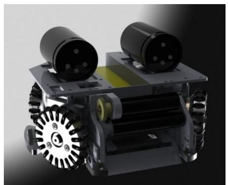
The mechanical system of small size robot consists of the wheels, the kicker, the dribbler and the motion system. Some problems in last version of MRL small size robots encouraged us to change the materials and mechanical design. The diameter of the robot is 179mm and the height is 149mm.The spin back system conceals 20% of the ball diameter in maximum situation. Different parts of our new mechanical design are described in the following. Fig. 27 shows our new mechanical design. The first version of the robot with this structure is produced and investigated in Iran open 2011 competitions. We hope to resolve the remained problems till world cup competitions in Turkey.
4.1. Wheels
The small size robot which has been designed and made last year, had four Omnidirectional wheels, but because of changing the motors, to use their best quality and to reduce the slip, we resized our wheels dimension. Calculating wheel diameter for new robots resulted in 29 millimeters which is 5 millimeters larger than the previous one. Thus, More O-rings can be used to make the Omni directional characteristics of the wheels which are made from Neoprene. Each wheel has twenty rollers which are designed thinly to embed into the carpet for more traction. Also, in order to create smooth motion, two ball bearings are fetched into each wheel. The robot's wheel has enough friction to drive the robot with acceleration even more than 3.5 m/s 2 .
Figure 28 shows our custom-made wheels. In this figure, every parts of the designed wheel in SolidWorks are depicted in the left side and the real manufactured one is in the right side. In this new design, the installation and opening of the wheels became more simplified. Also internal gear-head prevents entering the rug piles and disturbing the robot motion components.
The wheel body is made of Aluminum Alloy from 2008 to now. Further information about our progress in these years in mechanical design which are related to the wheel characteristics are presented in table I.
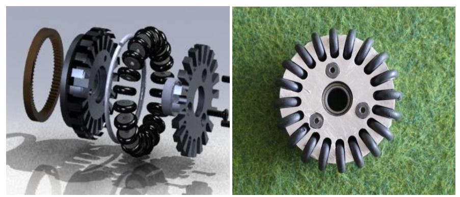
Table I. MRL wheel specifications from 2008 to 2011.
| Model | 2008 | 2009 | 2010 | 2011 |
|---|---|---|---|---|
| Number of wheels | 3 | 4 | 4 | 4 |
| Wheels diameter | 64 | 60 | 54 | 59 |
| Wheels thickness | 8 | 9 | 16 | 16 |
| Number of rings | 20 | 15 | 18 | 20 |
| Gears ratio | 1:5 | 1:4.4 | 1:4 | 1:3.6 |
| O-ring's material | Viton | Viton | Neoprene | Double seal Buna-N |
4.2. Kickers
The robot uses two kinds of kicking system, direct kick and chip kick. Each of them is divided in two part, solenoid and plunger. The magnetic plunger material is pure iron ST37. Because of the electromagnetic effect two separate parts are used in the cylindrical plunger. The custom-made cylindrical solenoid is used for direct kick which has ability to kick the ball up to 12 m/s. Last year our direct kicker was made from Aluminum alloy but the kickers were broken frequently during the matches. To solve this problem, we replaced it by Titanium Alloy for the new robot. Direct kick solenoid is located between kicking plates which are made from polyamide and aluminum.
As a second kicking system, MRL2011 has a custom-made flat solenoid. Because of space limitation with high performance chip kick we decided to reshape the solenoid from cylindrical to flat rectangular and placed in the front part of the robot. The chip kick has a 45 degree hinged wedge front of the robot which is capable of kicking the ball up to 6m before it hits the ground. The chip kicker is made from Aluminum Alloy 7075 which is enough strong to kick the ball. Chip kick system has a different plunger from direct kick; chip kick plunger is made from Steel with the thickness of 3.70mm.
In Fig. 29 different parts of the kickers in the robot construction are displayed. During previous four years, we have tried various materials to make the best mechanism for the kickers. Our experiences about this part in these years are summarized in Table II.
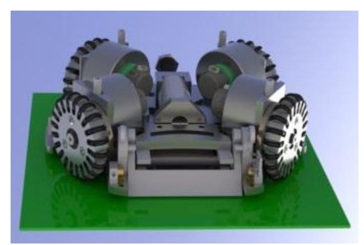
Table II. MRL kickers specifications from 2008 to 2011.
| Model | 2008 | 2009 | 2010 | 2011 |
|---|---|---|---|---|
| Cylenderical Solenoid | Plastic | Phenolic | Backlite | Backlite |
| Flat Solenoid | Plastic | Phenolic | Backlite | Backlite |
| Direct Kicker | Aluminum Alloy | Aluminum Alloy | Titanum Alloy | Titanum Alloy |
| Chip Kicker | Aluminum_Steel | Aluminum_Steel | Copper_Steel | Copper_Steel |
4.3. Dribbler
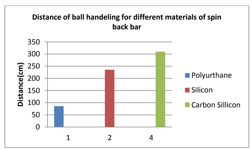
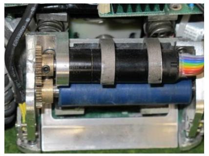
Dribbling system is a mechanism to improve the capability of ball handling. Dribbler is a steel shaft covered with a rubber and connected to high speed brushless motor shaft, Maxon EC16 Brushless, with 1:1 external gear ratio. The 5.4:1 planetary gear-head is attached to this motor. We examined several materials for dribbler bar, like Polyurethane, Silicon and carbon silicon tube. The results of examining different materials in this module are shown in Fig. 30. As it is observable from this figure, Carbon Silicon is selected for its higher capability in ball handling. When our supply voltage is 14.8V, replacement of 24V motors with 18V ones, increases the efficiency of our mechanism and reduces the losses.
To prevent the impact of ball contact with the spin-back, using a compliant object is necessary for suspension system at the back of the structure. Firstly, we applied two springs as shown in Fig. 31, but after some tests, a piece of sponge was preferred which is utilized in Iran open 2011 with acceptable performance too. We also added a servo motor to the dribbler mechanism to have ability of tuning the system in any situation in the future. We use a screw as a limiter, allowing the suspension system to swing backward with maximum of 7 degrees. This kind of suspension system, consisting sponge damper and servo motor, gives the ability of receiving the high speed moving ball in passing situation to the robot.
The sender and receiver of IR sensors are placed on two sides of the spin-back frame. This year to protect them from the impact of the ball or opponent robots, both sides of spin back arms are covered with small Aluminum plate. Another mechanism is designed to protect the motor from bumps which are shown in Fig. 31 too.
4.4. Motion system
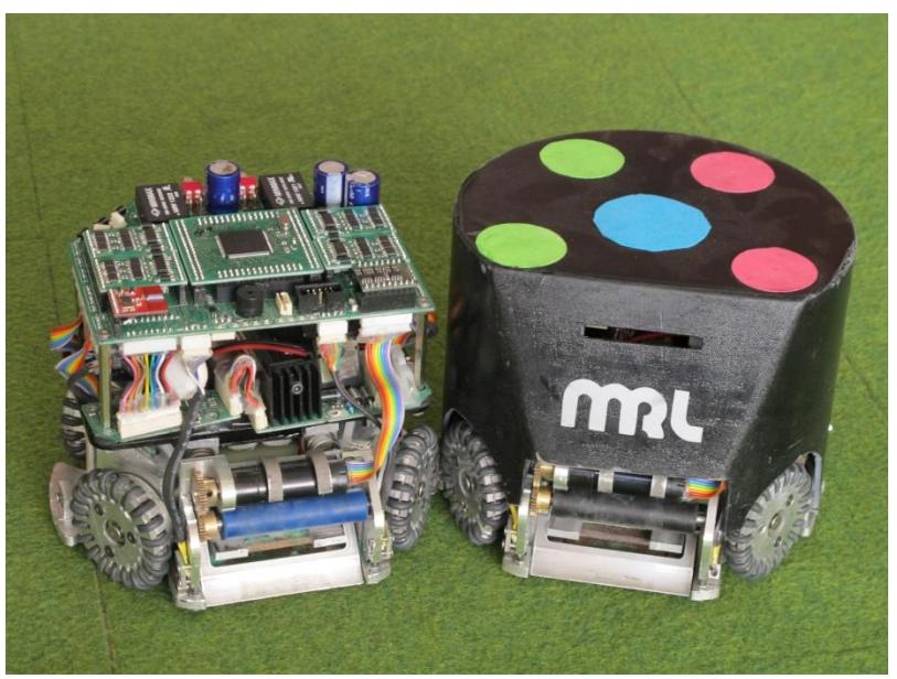
The robot uses brushless motor, 50 watts Maxon EC45 flat, in the driving system. The motion system uses external gear with ratio of 1:3.6. This kind of motor and the mentioned gear ratio can provide more acceleration and velocity than our previous one. The motor of robot is connected to a 360 CPR optical encoder for speed measurement. Each encoder is connected to the motors with a custom-made intermediate plate. We used 5mm thick Aluminum Alloy 6061 plate as a chassis. This plate connects all the parts together, such as motor's stand, direct solenoid and etc. Fig. 32 shows our robot in Iran open2011 competitions.
4 Motion Control
Control section contains two main parts; Motor control that concerns about each wheel of robots to work at the desired performance, and motion control on each robot to move on the desired trajectory with desired velocity profile.
5.1. Motor Control
As it is described in the hardware section, each wheel of a robot is derived by a MAXON™ EC16 - 50 watts motor. Torque is then transferred to the wheel by a gearbox with ratio 1:3.6. This motor is modeled by a first order linear system. Based on the coefficients derived from the data sheet [7], gearbox ratio and the PWM module gain, the overall model from the input voltage to the motor angular velocity is calculated as follows:
$$T(s) = \frac{2.06}{s+117} \tag{8}$$
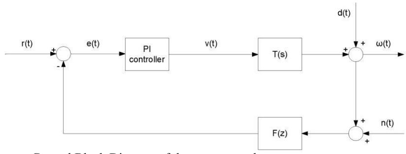
Figure 33 shows the control block diagram of the motor speed.
where is the desired angular velocity of the motor that is calculated in the ARM by the desired robot velocity in the body-fixed frame. is the input of the PWM that is generated by the PI controller. is the motor angular velocity. is the first order digital low-pass filter that is used to filter the measurement noise on the angular velocity measured by the encoder. ARM reads encoder data and sends new commands with sampling period equal to .
After converting digital filter to the continuous filter by Tustin method, see [8], the PI controller is designed by the root lucas method to achieve a closed-loop response with less than overshoot and settling time .
The main limitation on the closed-loop response speed is forced by the law pass filter. Suppose is the simple pole of the digital filter, then the minimum achievable settling time will be determined by (9)
$$\min t_s = 2\pi t_s \frac{1+z_0}{1-z_0} \tag{9}$$
Since is already set to filter the encoder output, we can decrease to reach less settling time. The minimum sampling period that is acceptable by the ARM is .
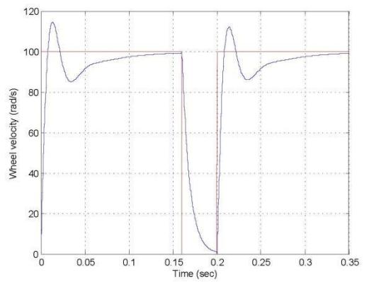
The closed-loop wheel velocity response to a usual step input are illustrated in figure 34.
5.2. Motion Control
One of the most important challenges in the small size robot soccer is the motion control, which means being in the desired position at the minimum time with sufficiently small error. To this goal, many teams in the recent years pay special attention on the motion control, e.g. [9] and [10]. The main approach that is proposed by Skuba, is modifying the kinematic static model of motion for robot and calculating the modified command based on the modified model. We extend this approach based on a dynamical model of motion.
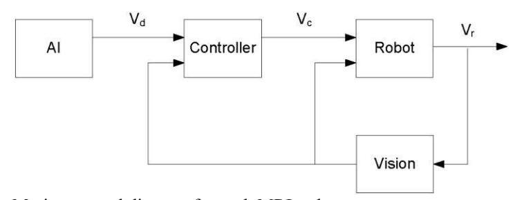
In general, AI module defines the best path from the current position to the desired position. Then, based on the maximum values for acceleration and deceleration, two trapezoidal profiles for the desired speed in the $X^E$ and $Y^E$ coordinates of the earth-fixed frame are generated. The desired speeds for the next time step in three coordinates are transformed to the body-fixed frame and send to the robot. We call this velocity vector, desired velocity $V_d = [v_x \quad v_y \quad \omega]^T$. It is necessary to force the robot to move on this desired speed. Unfortunately, if $V_d$ is directly used as a command velocity $V_c$, the robot real speed $V_r$ that is measured by vision system, could not reach the desired speed. This occurs because of different kinds of friction and uncertainties in the robot mechanic like deviation of the center of mass and other practical problems.
To overcome this drawback, a controller is required to construct a modified command based on the desired velocity $V_d$ to decrease the tracking error $e_{track} = V_d - V_r$ as much as possible. Figure 35 contains a block diagram schematic of the closed-loop system.
To obtain a suitable command, the first step is finding a model robot motion between the command speed and the real speed. In the latest work by Skuba in [9] this relation is supposed to be a static gain, so the modification is done by a feed forward control. We suppose a linear MIMO dynamical model for the robot motion as
$$\dot{V}_r = AV_r + BV_c + D \tag{10}$$
By this model, the next measured velocity of the robot is dependent on the current velocity and the command.
To complete the model (10) matrices A, B and D should be identified. This is done in the offline tuning phase by forcing the specified robot with different commands $V_c$ (at the first run ) and saving the robot velocity at each time. By Euler approximation to the differentiation (11) is obtained.
$$V_r(t+dt) = (dtA+I_3)V_r(t) + dtBV_c(t) + dtD$$ (11)
where is the sampling period of the vision system. By Kronecker product, the matrix equation (11) is transformed to an equation with a vector as an unknown term which should be found. The least square technique is then used to find unknown matrices , and .
Now the modified command for the current time named to make at the next sampling time is computed by (12).
$$V_c(t) = \frac{B^{-1}}{dt} { V_d(t+dt) - (dtA + I_3) V_r(t) - dtD }$$ (12)
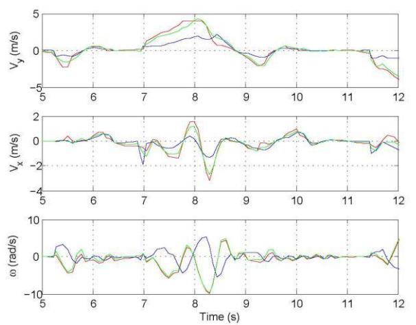
Equation (12) is a feedback control law. Figure 36 shows a trapezoidal desired velocity and the robot real velocity with and without controller (12).
Some remarks:
- Tuning phase can be done or continued online. In this case to avoid computation complexity and memory problem recursive least square can be used, for more details see [11]. By this online tuning, we reach to the adaptive version of the controller (11) that improves the robot motion during the game and considering the time variable parameters .
- Experiments shows that model (9) depends on the angular velocity . Thus, to get better results, we can compute , and for different and then fit a polynomial of to obtain , and . Although we hope that this extension makes the motion better, it is not tested yet.
- Another extension is using different values for , and in the acceleration and deceleration phases.
References
- A. Azidehak, M. Hoshyari, M. A. Sharbafi "Design and Implementation of Minimal Components Brushless DC Motor Driver for Mobile Robots" 2011 IEEE International Conference on Mechatronics, Istanbul, Turkey, (2011).
- Bakhshandeh, O., M., Sharbafi, "Modeling and Simulating of Omni Directional Soccer Robots" 2011 IEEE 3rd International Conference on Computer Modeling and Simulation (ICCMS 2011), Mumbai, India, (2011).
- Sharbafi, M. A., Hoshyari, M., Esmaeelpourfard, S., Bakhshandeh, O., HaajSeyedjavadi, E., Esmaeeli, D., MRL 2010 Team Description, In Proceedings of the 14th International RoboCup Symposium, Singapore, Singapore, (2010).
- Samuel, A. L., "Some Studies in Machine Learning Using the Game of Checkers". IBM Journal of Research and Development, no. 3, pp. 210–229, (1959).
- Sutton, R. Learning to Predict by the Method of Temporal Differences. Machine Learning, no. 3, pp. 9–44, (1988).
- Sharbafi, M.A. Lucas, C. Daneshvar, R., "Motion Control of Omni-Directional Three-Wheel Robots by Brain-Emotional-Learning-Based Intelligent Controller", Systems, Man, and Cybernetics, Part C: Applications and Reviews, IEEE Transactions on, vol. 40, no. 6, pp. 630-638, (2010).
- Maxon motor, Key information on maxon DC motor and maxon EC, Maxon Motor Catalogue, (2010).
- K. Ogata, Discrete-Time Control Systems, Prentice Hall; 2nd ed., (1995).
- J. Srisabye, et. al., "Skuba 2009 Extended Team Description", In Proceedings of the 15th International RoboCup Symposium, Graz, Austria, (2009).
- Y. Wu, et. al., "Extended TDP of ZjuNlict 2009", In Proceedings of the 15th International RoboCup Symposium, Graz, Austria, (2009).
- L. Ljung, System Identification: Theory for the User, Prentice Hall; 2nd ed., (1999).