Skuba 2011 Extended Team Description
Krit Chaiso, Kanjanapan Sukvichai
Department of Computer Engineering, Faculty of Engineering, Kasetsart University; Department of Electrical Engineering, Faculty of Engineering, Kasetsart University
Abstract This paper presents a detailed description of Skuba, a Small-Size League RoboCup robot team in addition to the team description paper. The robot system is designed under the RoboCup 2011 rules in order to participate in the RoboCup competition in Turkey. The low level and high level control of the SKUBA system are explained in each section.
1 Introduction
Skuba is a small-size league soccer robot team from Kasetsart University, which has entered the RoboCup competition since 2006. We got the championship from last two years from the RoboCup 2009 in Graz, Austria and 2010 in Singapore. Another championship is in April 2011 from RoboCup Iran Open 2011 in Tehran, Iran.
The robot system consists of two main components: the robot hardware and the software. The software makes strategic decisions for the robot team by using information about the object positions from the vision system. The global vision system run by the shared vision software, SSL-Vision, uses two cameras mounted over field. The software executes plans by calculating the robot actions and then sends the commands to each robot.
Our team has ten identical robots, six of them were built in 2008 and another four were built in 2009 with some minor changes in material and mechanical design. We are not planning to make any major changes to the design. The robot hardware is the same as used in last year.
This year, the main focus of this extended team description paper is to expand our control system. The control parameters are measured by automatic calibration process which simply uses the same procedure as the manual calibration does, but it's done automatically by the software.
1.1 Team Members
Kanjanapan Sukvichai : Control Theory and Supervisor
Krit Chaiso : AI Software and Team Leader
Chanon Onman : AI Software Nuttapol Runsewa : AI Software Khakhana Thimachai : AI Software Phawat Lertariyasakchai : AI Software Tanakorn Panyapiang : AI Software
Teeratath Ariyachartphadungkit : Electronics, Mechanics and Low level Firmware
Supavit Siriwan : Electronics and Mechanics
Peerapat Kittiboriluk : Mechanics
2 Robot Hardware
This section describes the robot electronics system that is used in driving system including the designs and components. Details about operations and algorithms are in the firmware section.
The robot consists of two electronics boards: the main board and the kicker board. The main board handles all of the robot tasks except kicking. The kicker board controls the entire kicker system.
2.1 Main Electronics Board
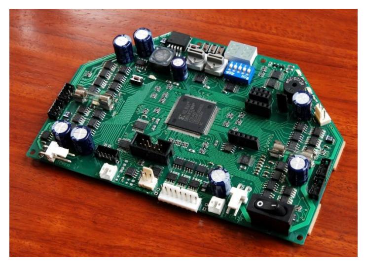
The board consists of a Xilinx Spartan-3 XC3S400 FPGA, motor driver, user interface, some add-on modules and debugging port. The microprocessor core and interfacing logic for external peripherals are implemented using FPGA in order to handle the low-level control of the brushless motor such as velocity and position control. The main electronics board receives commands from the main software on a computer. The board integrates the processing components together with the power components to keep the board compact and minimize wiring. With limited space, almost components are in small SMD packages. However, these components still large enough for hand soldering with conventional tools. Figure 1 show the main electronics board of the robot.
2.2 Motors
There are two types of motor in the robot, the driving motor and the dribbling motor, both are brushless motor. Each driving motor is a 30 watts Maxon EC45 flat motor with a custom back-extended shaft for attaching encoder wheel. The motor itself can produce a feedback signal from hall sensors for measuring wheel velocity. However, this multi-pole motor sends only roughly 48 pulses per revolution; therefore, this motor is equipped with an US Digital E4P encoder which have higher resolution of 1440 pulses per revolution. The dribbling motor is a high speed 15 watts Maxon EC16 motor. Despite a very low resolution of 6 pulses per revolution signal from hall sensors, the implementation of the PI controller is possible when running this motor at high speeds. The maximum speed of the dribbling bar is about 13000 rpm.
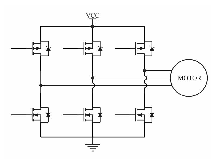
The motor driver is a three phase inverter circuit using complementary N and P channel power MOSFET in each phase. This configuration doesn't require bootstrap driver as in N-channel-only configuration. These MOSFETs are driven by MOSFET driver ICs to minimize switching loss. The motor commutation and PWM generation are described in the firmware section. Figure 2 shows the three-phase brushless motor driver circuit.
3 Robot Low Level Control
The main electronics board consists of a FPGA as a single chip central controller. The FPGA is embedded with a 32-bit processor, brushless motor controller, PWM generator, quadrature decoder, kicker board controller and onboard peripheral interfacing cores: SPI and UART. The processor runs at 30MIPS as same as oscillator clock speed. We use Altium Designer and Xilinx ISE software to generate, configure and debug these cores.
3.1 Brushless Motor Driver
The three phase inverter bridge is fed with signals from FPGA to provide commutation for each motor. These signals are ANDed with the PWM signal to vary the average voltage applied to the motor winding. The six steps commutation sequence is detected by three hall sensors in the motor. Both high and low side drivers are driven by PWM signals to control the torque applied to the motor.
3.2 Motion Control
The robot employs a PI controller as a motion controller, one controller for each motor. The control loop executes 600 times per second using velocity feedback from the encoder in driving motor and hall sensors in dribbling motor. The proportional and integral gains are manually hand-tuned. The computer sends a velocity for each DOF: x-y axis and rotation axis. Then, converted to each wheel velocity and sent to the PI controller. The output from the controller is sent directly to the PWM controller.
3.3 Over-current Protection
General problem when driving the inverter bridge is the shoot-through current. This current is caused by turning on one side of the driver immediately after the other side of the driver has been turned off, because the MOSFET turn-off time is usually higher than the turn-on time. This situation occurs when the motor is reversing direction, which can be prevented by adding a small delay time between each high and low side driver signal.
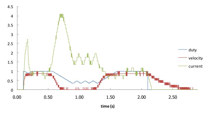
Many of robot skills use the dribbler. Some ball stealing skills can cause dribbling motor to stall when the dribbling bar is contacted with the opponent robot. The stalled motor consumes very high current and often burn the fuse out. This over-current situation can be detected by a current sensor and can be prevented by limiting a PWM duty cycle until the current drop below the safe motor operating current. Figure 3, depicts the motor stalling situation. When the motor stalled, the motor current increased and dropped in a short time due to limited duty cycle. The motor current is controlled around the threshold while the motor is stalling.
3.4 Torque Control for Maxon Brushless Motor
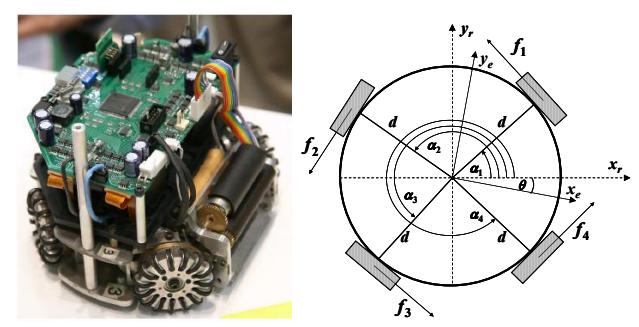
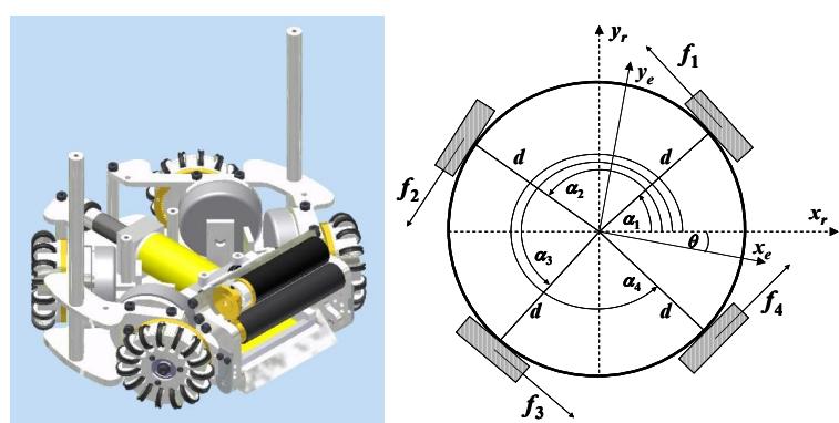
The dynamics of a robot is derived in order to provide information about its behavior. Kinematics alone is not enough to see the effect of inputs to the outputs because the robot kinematics lacks information about robot masses and inertias. The dynamic of a robot can be derived by many different methods such as Newton's law and Lagrange equation. Newton's law is used to solve the robot dynamic equation. The interested mobile robot is consisted of four omni-directional wheels as shown in figure 4. Newton's second law is applied to robot chassis in Fig 1 and the dynamic equation can be obtained as (1) though (3).
$$\ddot{x} = \frac{1}{M} \left( -f_1 \sin \alpha_1 - f_2 \sin \alpha_2 + f_3 \sin \alpha_3 + f_4 \sin \alpha_4 \right) - \vec{f}f \Big|{x}$$ (1)
$$\ddot{y} = \frac{1}{M} (f_1 \cos \alpha_1 - f_2 \cos \alpha_2 - f_3 \cos \alpha_3 + f_4 \cos \alpha_4) - \bar{f}f \Big|{y}$$ (2)
$$J\ddot{\theta} = d(f_1 + f_2 + f_3 + f_4) - T_{trac} \tag{3}$$
where,
$\ddot{x}$ is the robot linear acceleration along the x-axis of the global frame $\ddot{y}$ is the robot linear acceleration along the y-axis of the global frame
M is the total robot mass
$f_i$ is the wheel i motorized force
$\vec{f}_f$ is the friction force vector
$\alpha_i$ is the angle between wheel i and the robot x-axis
$\ddot{\theta}$ is the robot angular acceleration about the z-axis of the global frame
J is the robot inertia
d is the distance between wheels and the robot center
$T_{trac}$ is the robot traction torque
![[Figure caption not provided in source]](/tdps/soccer_smallsize__2011__Skuba/_page_6_Picture_15.jpeg)
Robot parameters
| M | 1.5 kg |
|---|---|
| J | $0.0192 \text{ kg/m}^2$ |
| d | 78.95 mm |
| $[\alpha_1,\alpha_2,\alpha_3,\alpha_4]$ | [33,147,225,315] degree |
| r | 25.4 mm |
| $V_{cc}$ | 14.8 V |
| $k_m / R$ | $0.02125~\text{Nm}/A\cdot\Omega$ |
| $k_m/(R\cdot k_n)$ | $0.0005426$ $Nm \cdot V \cdot s / A \cdot \Omega \cdot rad$ |
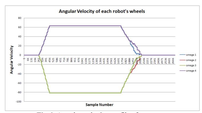
Trapezoidal trajectories for robot are generated by using the robot kinematic equation with different conditions. The experimental set-point angular velocity is shown in figure 6.
The experimental parameters
| Case | () 0 | x | x |
|---|---|---|---|
| 1 | 90 | 2 | 3 |
| 2 | 90 | 1.5 | 2 |
| 3 | 45 | 0.8 | 1 |
| 4 | 0 | 0.8 | 1 |
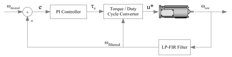
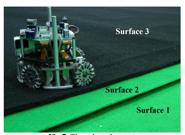
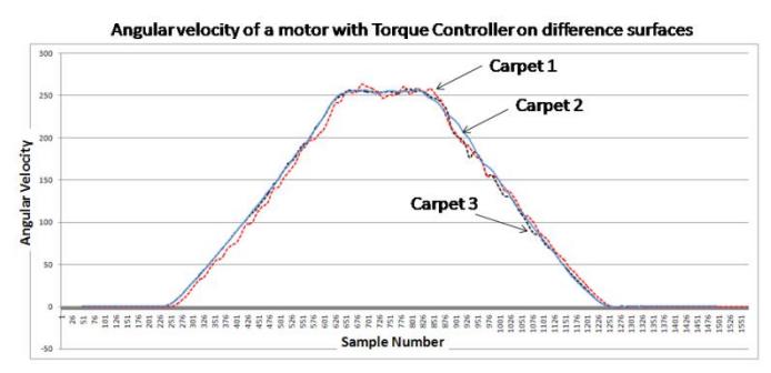
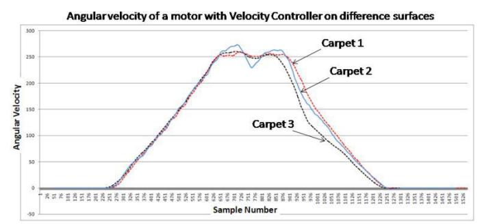
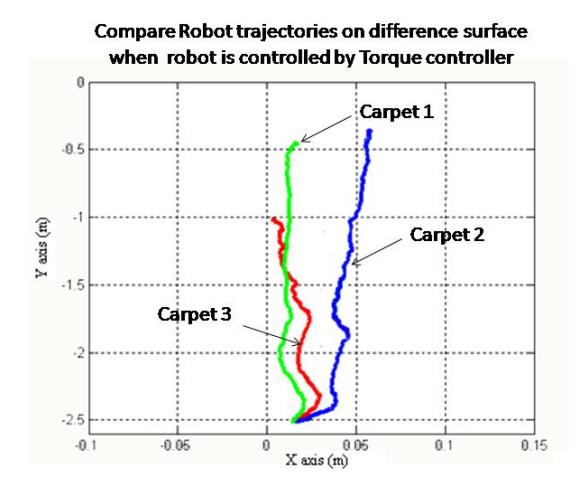
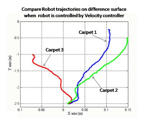
The output angular velocity of motors are collected and compared with the output from same motor but different carpets. Figure 8 shows the output angular velocity of a motor which is controlled by the torque controller while figure 9 shows the output angular velocity of a motor controlled by regular velocity controller. From the experiment, a motor with torque controller can maintain its velocity when the surface frictions are changed. For a motor with normal velocity controller, the output is swing dramatically when it runs on different surface. The result shows that a motor with torque controller has a better tracking response than a motor with velocity controller especially when the motor is breaking.
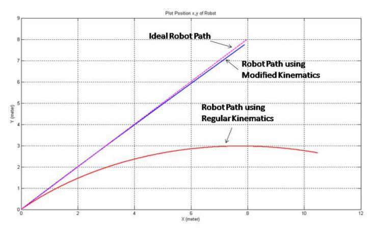
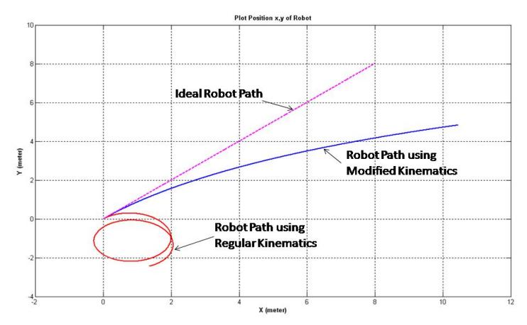
3.5 Modified Kinematic
4 Robot High Level Control
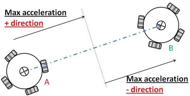
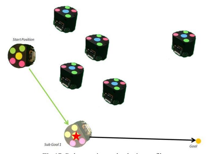
ControlModule receives predicted vision from VisionModule and destinations from StrategyModule and makes robots go to those destinations. So, the essential component of ControlModule is a path planning algorithm. Since the World RoboCup 2008 at Suzhou[4], we have made use of the "Real-Time Randomized (RRT) Path Planning for Robot Navigation" for default path planning algorithm and use of the "Sub Goal Path Planning" for fast move planning algorithm.
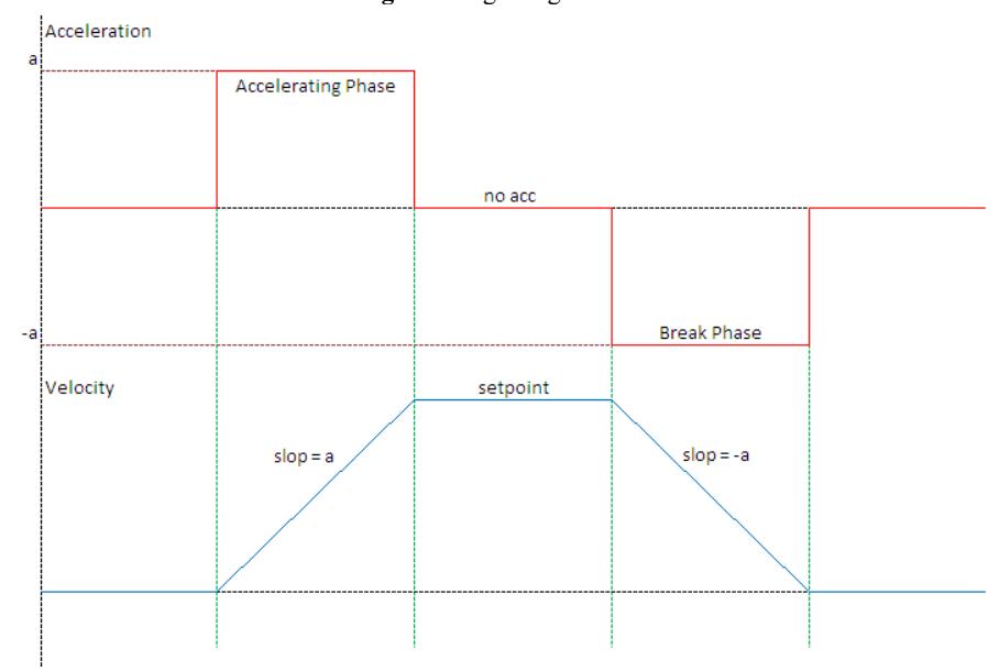
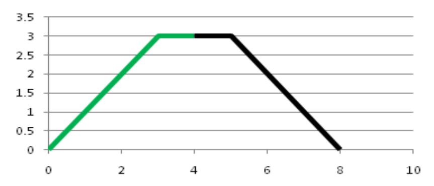
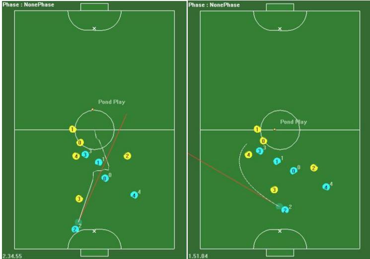
After the ControlModule get command to navigate robot from the start point to the end point, the ControlModule will find the path (RRT or Sub Goal) by using start position, end position, initial velocity along x and y axis and direction of starting point and ending point. The result path will be calculated the usage time in order to use this information generates the velocity command which will be sent to the robot. Sometime the velocity is limited by the maximum acceleration of the robot. The velocity command is generated separately to the every point along the trajectory according to the frame rate. Each frame has its own velocity command. If there are any obstacles block the robot path, the path planning will be spited to small straight line to avoid collision. The velocity profile is generated by using Bang-Bang algorithm as shown in figure 15 and 16. Final motion of the robot and robot velocity profile are shown in figure 17 and 18 respectively.
5 Conclusion
Our system has been continuously improving since the beginning. Last year, we introduced some improvements about the low level motion controller and the robot hardware. The new calibration software is fully testes in RoboCup 2010 and it greatly reducs the amount of team setup time which allowed us to focus more on the strategic planning. The software which runs the robot team was built in 2006 and improved each year. It has given us very successful competition results for the last several years, the results are summarized in table 3. We hope that our robot team will perform better in this year and we are looking forward to sharing experiences with other great teams around the world.
Competition results for Skuba SSL RoboCup team.
| Competition | Result |
|---|---|
| RoboCup Thailand Championship 2005 | 3rd Place |
| RoboCup Thailand Championship 2006 | Quarter Final |
| RoboCup 2006 | Round Robin |
| RoboCup Thailand Championship 2007 | 3rd Place |
| RoboCup Thailand Championship 2008 | 2nd Place |
| RoboCup 2008 | 3rd Place |
| RoboCup 2009 | 1st Place |
| RoboCup China Open 2009 | 1st Place |
| RoboCup 2010 | 1st Place |
| RoboCup Iran Open 2011 | 1st Place |
References
- K. Sukvichai, P. Wasuntapichaikul and Y. Tipsuwan, "IMPLEMENTATION OF TORQUE CONTROLLER FOR BRUSHLESS MOTORS ON THE OMNI-DIRECTIONAL WHEELED MOBILE ROBOT", ITC-CSCC 2010, Pattaya, Thailand, 2010, pp 19 22.
- J. Srisabye, P. Wasuntapichaikul, C. Onman, K. Sukvichai, et al. "Skuba 2009 Extended Team Description," Proceedings CD of RoboCup 2009.
- K. Sukvichai, P. Wechsuwanmanee, "DEVELOPMENT OF THE MODIFIED KINEMATICS FOR A WHEELED MOBILE ROBOT", ITC-CSCC 2010, Pattaya, Thailand, 2010, pp 88-90.
- P. Wasuntapichaikul, J. Srisabye, C. Onman, K. Sukvichai, "Skuba 2010 Extended Team Description of the World RoboCup 2010", Kasetsart University, Thailand, 2010.