ER-Force Team Description Paper for RoboCup 2012

Jan Kallwies, Simon Dirauf, Philipp Nordhus, Simon Kerschbaum, Stefan Friedrich, Michael Bleier

Robotic Activities Erlangen e.V. Pattern Recognition Lab, Department of Computer Science University of Erlangen-Nuremberg Martensstr. 3, 91058 Erlangen, Germany

http://www.robotics-erlangen.de/

Abstract This paper presents an overview description of ER-Force, the RoboCup Small Size League team from Erlangen, Germany. The current tracking algorithms and processing stack is outlined. The main part of the paper gives a detailed description of the model-based motion control implemented on the robots and trajectory planning and position control algorithms used on the external computer. Furthermore, upcoming changes and improvements are outlined.

1 Introduction

In this paper the motion control and trajectory planning components of the RoboCup team ER-Force is presented. The team, located at Friedrich-Alexander-University of Erlangen-Nuremberg in Germany, participates in RoboCup competitions since 2007. This year focus lies on improving the motion control algorithms to provide faster reaction times and on adjusting both the position and the orientation of the robots. In section 2 the tracking algorithm and the organization of data flow in the system is presented. The design and implementation of the control loops for velocity and position as well as the basic planning algorithms for valid trajectories is illustrated in section 3.

2 State Estimation and Tracking

The task of object detection has been greatly simplified by the introduction of SSL-Vision [1]. This software is able to identify objects reliably in most situations. However, since it does not include any form of tracking, detection will fail eventually. For instance, the ball will not be detected if it is occluded by a robot due to perspective projection. Furthermore, among other situations, fluctuations in lighting conditions may render an object temporarily invisible.

It is necessary for the control algorithms presented in section 3 to have valid data on each iteration. If no position data is available at any iteration, the software will fail to generate movement commands. Therefore, a tracking system has been implemented. The well-known Kalman Filter [2] is applied to filter noise in the detection data from SSL-Vision. This algorithm also tracks objects, i.e. it provides an estimate of the current position and velocity even if there are no new measurements available.

For optimal control the delay between receiving new vision data and the transmission of the control action to the robots has to be kept as small as possible. Moreover, for easier analysis and design of the control algorithms it is preferred that all low-level control loops run with a fixed frequency. SSL Vision does not provide any guarantees about the timing of the vision data packets since both cameras (or even all four with a large field) are triggered independently and the processing threads are not synchronized. Hence, the information from each individual processing stack is received with a small, non-constant delay and motion control cannot simply be executed whenever new vision data is available. In this implementation, a dedicated thread first runs the tracking algorithm and directly afterwards motion control calculations. As a compromise, this thread is triggered with a fixed frequency of 120Hz which relates to approximately the double camera frame rate. Upon activation the thread first iterates over all vision packets received since the last activation, in chronological order. For each packet, all currently tracked objects are predicted to the time when the packet was received. This receive timestamp is calculated by subtracting the SSL-Vision runtime from the time when the packet was received on the control computer. Any additional latency by Firewire and UDP communication is neglected. After prediction, each object is updated with the measurements from this vision packet. When all vision packets have been processed, all filters are predicted to the current time. Finally, motion control is run with this estimated data.

3 Motion Control

Motion control is one of the most important areas in the Small Size League due to the very fast and agile robots. This topic is already addressed in several works, e.g. [3] or [4].

In this paper, however, a new approach for motion control, in particular the velocity control on the robot, is presented.

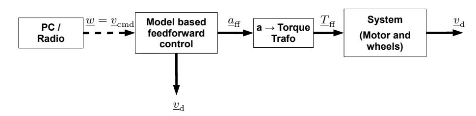
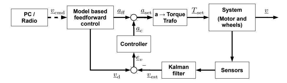
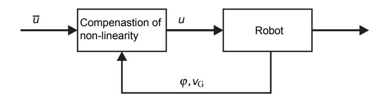
The entire motion control system is divided into two parts, the velocity control processed on the robot and the position control on the supervising computer. The position control's main purpose is to calculate the way and the corresponding velocities of the robot through the waypoints generated by the path-finding in an adequate way. The desired velocities are subsequently sent to the robot by radio. Finally, the velocity control on the robot ensures that the robot motion complies to the desired velocity.

3.1 Velocity Control

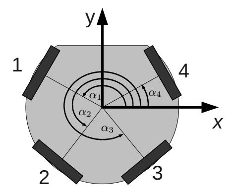
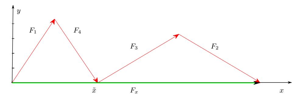
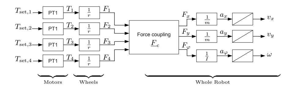
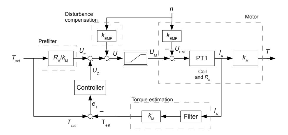
The velocity control system takes care of the velocity in x- and y-direction as well as the rotational speed of the robot. The corresponding coordinate system of a four-wheeled robot can be seen in Fig. 1.

Fig. 1. Model of the robot including the axes and the angles of the motors

Fig. 2. Structure of the feed-forward system for the velocity control

Fig. 3. The model-based feed-forward control

Fig. 4. Example trajectories generated by the model-based feed-forward control

Fig. 5. The desired force in x-direction $F_x$ divided into the four motor forces

Fig. 7. Structure of the torque control per motor

Fig. 8. The complete structure of the velocity control for the robot

3.2 Position Control

Trajectory Planning The algorithm is implemented in the scripting language Lua [7] to avoid the need for recompilation of the source after implementing changes. This helps to quickly test modifications of the code.

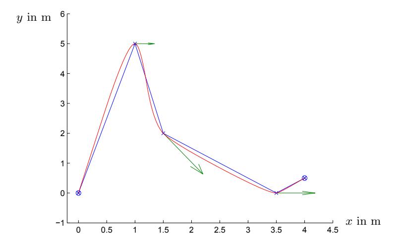
The trajectory starts at the current position of the robot. The pathfinding generates waypoints which shall be passed by the robot in successive order. In addition it determines the velocity and rotational orientation which the robot should have, when it reaches the final waypoint. To connect all waypoints with a feasible trajectory, the velocity and its direction at every waypoint must be known.

First, all waypoints are connected via linear intercepts. The time needed to get from one waypoint to another is estimated on the basis of the length of these segments. The direction of the velocity at one waypoint is orthogonal to the angle bisector of the two lines which meet at one waypoint. The absolute value of the velocity is limited by three factors. If the waypoint is close to the previous one, the velocity should be similar to the velocity of the previous waypoint, as the acceleration is limited. If the waypoint is close to the last waypoint, the velocity is limited for the same reasons. Furthermore, we take the angle between the two lines, which meet at the waypoint, into account. If the angle is big, the velocity is close to the maximal velocity. With smaller angles a smaller velocity is chosen.

The robot shall rotate permanently and reach its final rotational orientation and its final position at the same time. This way a rotational orientation can be assigned to each waypoint.

The linear connection between two neighbouring waypoints is divided into two parts with the same length. The acceleration vector is constant inside of each part. The acceleration in one dimension (x, y and rotational) can be calculated independently from the other two accelerations. The values of the accelerations are completely determined by the boundary conditions.

The whole method is visualized in Fig. 9.

Fig. 9. The waypoints are connected via linear intercepts, a velocity vector is calculated for every waypoint, and all waypoints are connected in a final step using splines.

Fig. 10. The linearized system consists of the compensating filter and the dynamics of the robot

4 Conclusion

Tests have shown that a well-performing tracking system increases the accuracy and reliability of the SSL-Vision detection. The presented algorithm has already proven to be very stable, and therefore reduces the dependency on a perfect vision calibration.

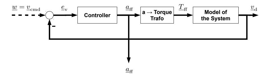
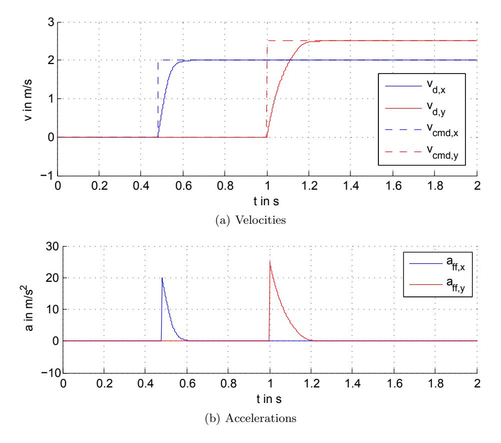
The motion control algorithms achieve a better command response by applying additional feed-foward control rather than common feedback-only. To reduce development time the algorithms have been verified in MATLAB/Simulink.

References

Zickler, S., Laue, T., Birbach, O., Wongphati, M., Veloso, M.: Ssl-vision: The shared vision system for the robocup small size league. RoboCup 2009: Robot Soccer World Cup XIII (2009) 425–436
Kalman, R.E.: A new approach to linear filtering and prediction problems. Transactions of the ASME – Journal of Basic Engineering 82 (Series D) (1960) 35–45
Chaiso1, K., Ariyachartphadungkit, T., Sukvichai, K.: Extended team description 2010 paper team skuba. (2010)
Umeno, T., Hori, Y.: Robust speed control of dc servomotors using modern two degrees-of-freedom controller design. IEEE Transactions on Industiral Electronics 38(5) (1991) 363–368
Grotjahn, M., Heimann, B.: Model-based feedforward control in industrial robotics. The International Journal of Robotics Research 21(45) (2002)
Oguntoyinbo, O.: PID Control of Brushless DC Motor and Robot Trajectory Planning and Simulation with MATLAB/Simulink. PhD thesis, Vaasan Ammattikorkeakouluuniversity of Applied Sciences (2009)
Ierusalimschy, R.: Programming in Lua. Lua.org (2006)