ZJUNlict Extended TDP for RoboCup 2012

Yonghai Wu, Penghui Yin, Yue Zhao, Yichao Mao, Qun Wang, Rong Xiong

National Laboratory of Industrial Control Technology Zhejiang University

http://www.nlict.zju.edu.cn/ssl/WelcomePage.html

Abstract This paper summarizes the details of ZJUNlict robot soccer system we have made since participated in Robocup2004. In this paper we will emphasize the main ideas of designing in the robots' hardware and software systems. Also we will share our tips on some special problems.

1 Introduction

Our team is an open project supported by the National Lab. of Industrial Control Technology in Zhejiang University, China. We have started since 2003 and participated in RoboCup 2004-2011. The competition and communication in RoboCup games benefit us a lot. In 2007-2008 RoboCup, we were one of the top four teams in the league. We also won the first place in Robocup China Open in 2006-2008 and 2011.

Our Team members come from serveral different colleges, so each member can contribute more to our project and do more efficient job.

Team Leader Yonghai Wu (AI) Team Member – AI: Penghui Yin, Yue Zhao, Qun Wang – Electronic: Yichao Mao, Yi Xuan, Xiaohe Dai and Yifan Shen

2 Hardware Architecture

2.1 Robot

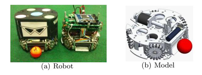
Components of the Robot Our robots are equipped with 4 omni-directional wheels. Each is driven by a 30 watt brushless Maxon motors which help our robot run with about 3.0m/s and 6.0m/s² . The reduction ratio of the gearbox with internal spur gear is 4:1. Besides there are three major machinery devices: a dribbling device, a shooting device and a chipping device. We redisigned the omni-wheels to reduce the friction between the small passive wheels and the driving wheel so that our robot's movement is smoother. We spend a lot of time testing the dribber materail in order to choose a satisfactory one. The robot is shown in Figure 1(b).

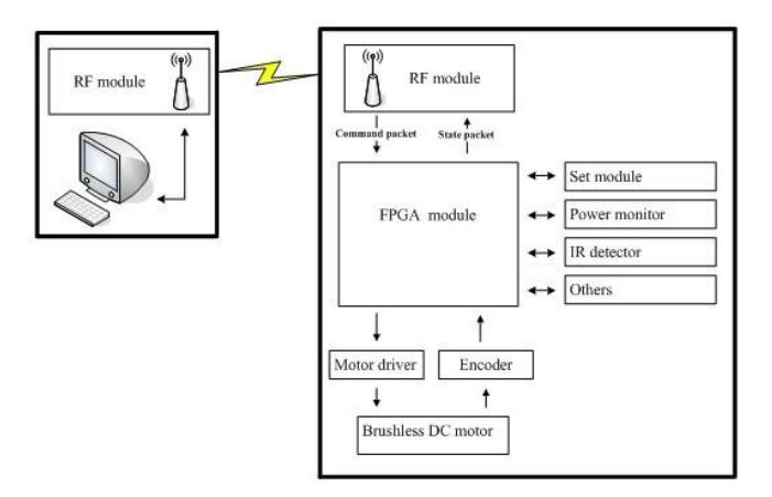
Our circuit architecture is FPGA based all-in-one solution as the central processor module. Our motor driving part is a stable module based on MC33035, which has been developed to complete the four years since 2007 in Atlanta.

There is an encoder module to form a local feedback control loop. A commercial wireless module based on nRF2401 is used on our robot. Meanwhile, we develop a new communication system between the PC and robots. We choose two smaller capacitors with higher voltage, to achieve a better result. They will help us save more power and permit several shots in short intervals. In addition, we have set module, power monitor module, IR detector module, and so on, in order to complete the functions of our robots. We use Protel Altium Designer 6.0 to layout the PCB board.

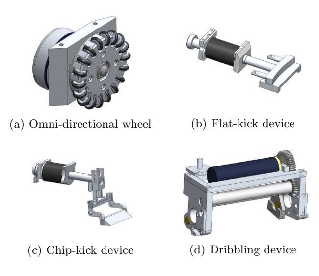
Mechanical Design Omni-directional Wheel Design Each wheel is composed of a big aluminous wheel with 18 grooves distributed equably in Circle, there is a small wheel founded with PM in every groove. Similarly, there is a groove in the small wheel, covered by a o-ring. The omni-directional wheel is shown in Figure 3(a) In RoboCup 2008, the wheel exhibited some problems, such as large gap and friction. Now the wheel is redesigned in some details, and receives a perfect performance. Except the wheels, we do not change a lot in the other parts. To improve the manufacture precision, we make all the parts with CNC machine tools.

Shooting Device Design The robot's shooting device is the primary method of both scoring and passing. It is made up of a an electromagnet and a simple mechanical structure. The electromagnet is made by ourselves and is calculated accurately in advance. It is drive by two big capacitors which is fixed on the floor board above. Since RoboCup 2007, we are pleased with our shooting devices and don't change a lot. It is shown in Figure 3(b). The shooting device can give the ball a maximum velocity of 10m/s. In the match, it is controlled by the circuit, the time and the force of kicking the ball is also in charge. This part of the robot is usually cooperate with others, such as the chipper,the dribbler.

Chipping Device Design The chipping device allows the robots to pass the opponent by kicking the ball into the air. As same as the shooting devices, it is also drive by two capacitors, the method to control it is also the same. It is shown in Figure 3(c). When the chipping device works, the shovel close to the ground can chip the ball to a maximum height of 0.8m and a maximum length of 3.2m. The angle of the shovel and the height between the chipping pole and the ground influence the performance most. When the ball falls to the ground, it is a litter difficult for the partner to get the ball steadily and quickly. Because of the elasticity of the ball and ground both play important parts.

Dribbling Device Design The dribbling device is the assembly that controls the ball. It is designed to stop a ball, control it and prevent losing it. The dribbling device is drive by a motor, accelerated by a pair of gears. A stick swathed with a special pipe circum gyrates when the ball comes close to the robot or it must compete for the ball with the opponent. From Robocup 2006 at Bremen, we found that the ball controlling ability is not very satisfactory, these years, we have tried many ways to improve it. We get a lot of experiences, receive a much better result now. It is shown in Figure 3(b). The higher rotate speed the motor circum gyrate, the bigger force the ball is given, but on the other hand, the ball will be easier to lose control. To get a better effect, we redesigned the limit device, besides we spend a lot of time choosing the material.

Electronic Design

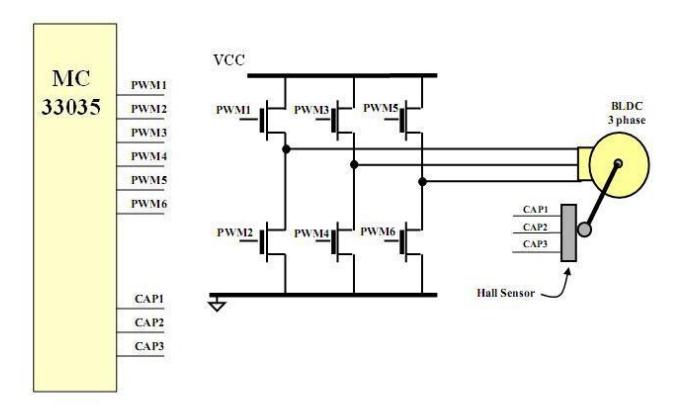
Driving Peripheral Design There is a local feedback control loop on the robot. Motor driving module based on a self constructed verilog module which consists of a rotor position decoder for proper commutation sequencing, temperature compensated reference capable of supplying sensor power, frequency programmable saw tooth oscillator, three open collector top drivers, and three high current totem pole bottom drivers ideally suited for driving power MOSFETs, Can Efficiently Control Brush DC Motors with External MOSFET H-Bridge.( Figure 4)

Communication Peripheral Design Our communication system is based on the module of NRF2401. NRF2401 is a single-chip radio transceiver for the world wide 2.4 - 2.5 GHz ISM band. The transceiver consists of a fully integrated frequency synthesizer, a power amplifier, a crystal oscillator and a modulator. Output power and frequency channels are easily programmable by use of the 3-wire serial interface. This year, a new communication system has been developed to reach better results. The new communication system is based on two RF modules on the robot. They were two separate modules, respectively charging for receiving and sending. Compared to last year, data transferred from the pc to robot, is encoded to a larger packet. All of the robot on the ground can receives the same packet at the same time, and pick up the right information with the numbers of themselves. the right information picked up from the large packet includes the speed of every wheels, shoot or chip command, the number of robot. Thus, every robot can receive the order without delay. Meanwhile the robots can send a packet to the pc. However, there is only one robot can send packet that contains useful information to pc. The PC can receive information from the robot without any delays. So the command sent from the pc can be implemented more effectively and timely.

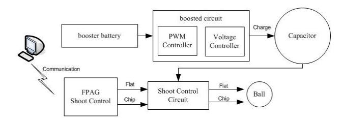
Shooting Peripheral Design Compared to previous years, our Shooting system ( Figure 5 )is not changed too much this year. Our boosted circuit includes a PWM control module and voltage control module, to control the boost capacitor voltage. FPGA sent chip or flat shoot signal, through control circuit for chip or flat shoot. However, we choose two smaller capacitors with higher voltage, to achieve a better result. The kicks are driven by two 4700uF capacitors charged to 190V . The kicker can give the ball a maximum velocity of 10m/s. With the increased voltage, the velocity will be faster.

3 Emebedded Software

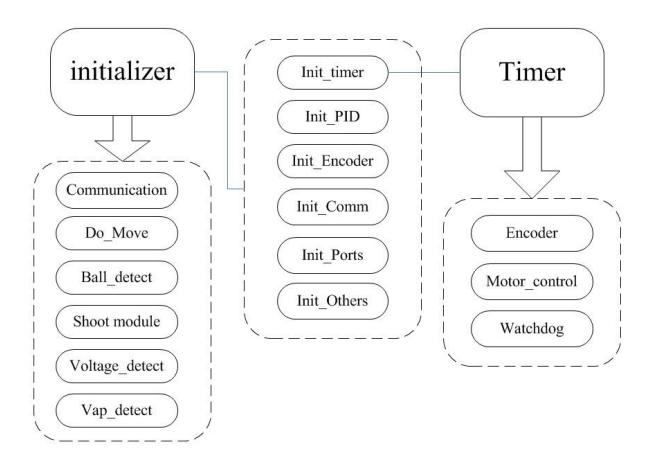
Since RoboCup 2007 in Atlant, Our circuit architecture use the NiosII as the central processor module which is a soft IP provided by Altera company matching at QuartusII9.1 and NiosII9.1 software programming environment. The overview of our embedded software flow is show in Figure 6.

3.1 Motor PID Control

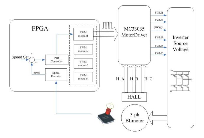
About the encoder module, we use a 512 gratings encoder with a decoder constructed by Verilog. It will count how many gratings it has detected in 2 ms, and then translated to the angular velocity of the motor, while it determine the direction of the velocity by phase difference between channel A and B which are quadrature signals shifted by 90. Based on the velocity we detect and the set velocity we desire, we can caculate the expected PWM duty with PI algorithm and the send it to the motor control module.

Based on our motor driver module ( Figure 7 ), we use an incremental PID algorithm, real-time code set encoding to read the speed of motor for PI and PID control, so that motor speed can reach the stable speed settings. About the encoder module, we use AM512, which is a compact solution for angular position sensing. The IC senses the angular position of a permanent magnet placed above the chip. So we put the permanent magnet on the motor, when the motor rotation, FPGA board will receive the Incremental signal from the encoder module. There are two signals for incremental output: channel A and channel B. Signals A and B are quadrature signals, shifted by 90. The speed of the motor can be count by the signals.

4 AI System

4.1 Strategy Hierarchical Architecture

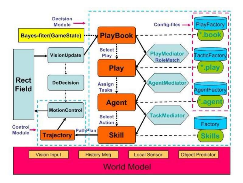
The AI module for our off-board control system is shown in Fig. 8. It is the brain of planning strategy and coordination among robots in both attack and defense mode. The whole system is composed of world model, decision module and control module.

With the bayes-based filter evaluating the game status, the decision module selects appropriate play during the match in state of continuity well. Besides, the decision module is rebuilt in a hierarchical style. The plays focus on coordination between teammates, while the agents emphasize on planning skills for the assigned single task from the corresponding plays. The skills are vital for good ones, contributing to executing tasks with high efficiency. Both play-level and agent-level are configured with Config-files, and will be detailed in next section. The control module is composed of path planning and trajectory generation. It takes RRT algorithm to find a feasible path and Bangbang-based algorithm to solve two-boundary trajectory planning. The world model provides all the information in the match while the decision module will feedback to the predictor in world model. Thus, the close loop system adjusts all agents behavior according to the change of the environment in real time. More details are shown in ZjuNlict2012TDP [2].

Game State Evaluation A right evaluation of game status plays an important role in the match. For the complexity of game situation, it's really a troublesome work. We consider a comprehensive view of the observation information, the strength of the rivals as well as the strategy we take to realize the evaluation. Our new method is based on the Bayes Theory [6], which gives a creative combination of the observation information and the historical strategy feedback.

Algorithm Bayes filter p(xk,uk,zk) for all xk do p(xk) = P xk p

               xk|uk, xk−1

                            p

                               xk−1

p(xk) = ηp zk|xk,

                   p

                     xk

end for

Fig. 9. General Algorithm for Bayes-filter

Fig. 9 depicts the basic Bayes Filter Algorithm in pseudo code form. our current method owns two main features:

• More stable: The evaluator gives more appropriate analysis of game state, even though there come momentary errors in observation information, and helps to reduce the perturbation of the strategy while strengthens the continuity of the strategy.
• Well targeted: Variable initial values of prior probabilities p(xk|uk, xk−1) in the algorithm accustomed to different characteristic teams, making it more convenient to configure the attacking and defending strategy in a more flexible way.

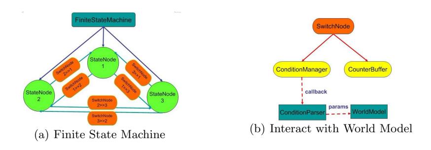
Finite State Machine This year, we mainly focus on script configuration to control robot behavior by a unified FSM-based mechanism, as is seen in Fig. 10(a). Every state node will link with the world model by using a condition parser contained in the connected switch node. The switch conditions are written in the external scripts and could be queried through internal world model.

Play Our AI module is implemented using a play-based approach. Each play represents a fixed team plan, in which each team group has a collaborating mission to perform and that group may have variable agents to execute. We can also consider the play a coach in the soccer game. The plays can transfer to each other, and the group for each agent can change too. As mentioned above, plays are designed and implemented with the unified FSM module. Plays are composed of many parts, such as applicable condition, evaluating score, roles, finite state machine and role tasks similar to CMU's STP [3]. These parts can all be configured by external scripts.

Agent Agent is performed as robot behavior which is assigned by play to control robot to perform a specific action such as manipulating ball to zone, passing the ball to a teammate, scrambling ball from opponent, getting ball. The agent first select a best proper team member according to the assigned zone and task which receive form play, then selects a proper skill for the team member performing the assigned behavior in every execution cycle and finally generates the best target for robot action. For example, in the shooting task it will be the best shoot point on opponent goal line.

Skill Skill is a set of basic knowledge for every agent, such as how to move to a point, how to get the ball and kick. Some skill generates a next target point of the specific path which will be passed to the navigation module for finally generating a avoiding collision path. Some skill will direct generate the speed trajectory for some special behavior such as pulling the ball from a opponent front. Each of skills has different main idea of generating path for robot, intercept the ball skill is different from move to point skill in many ways. We can test each skill independently for the best performance for each of skills.

4.2 Latency Measurement

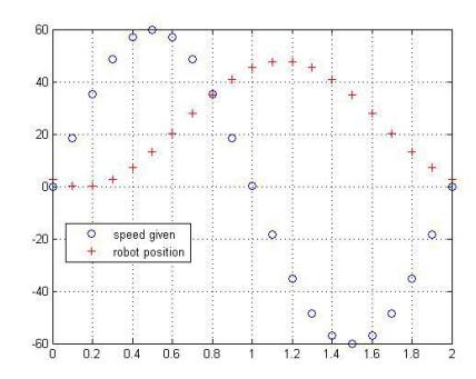
Because of the network transmission and image processing time cost, the AI module generated command received by robot will be later than the time camera captures this frame image. But when making decision we should take account of the state in which the robot just receives the motion command. So we must predict all of objects state in the field such as ball, our member and opponent in this latency duration (Figure 11).

In prediction routine, we must first know the system latency which starts in image capture and ends in the time command received by robots. We designed a easy experiment to measure this latency time. Detail of the experiment routine is show in following:

• 1. Make a robot stop in field, log this initial position
• 2. in the frame t we send a direct velocity along x axis which magnitude is k1sin(k2t), where t is the sample (or send) cycle.
• 3. At the same time we log this velocity command and robots new position
• 4. Without system latency, when the command speed accelerate to reach its maximum value, and then decelerate to zero, the robot just moves to the farthest distance away its origin position in positive direction. While command is negative, the robot goes back to its origin position.
• 5. Considering the system latency, when the command is send, it is after some time that robot will receive this command. So the time when command reaches zero doesnt synchronize the time when robot moves farthest.
• 6. Plot the robot position and command velocity magnitude in figure 11, we can see the difference between the time when the robot moving distance reaches its maximum value and the time when sending speed is zero.

Using this method we can get our system latency is about 4-5 frames (one frame is 1/60 s).

4.3 Path Planning

Path planning is an important issue in the mobile robot domain, we try to find a proper algorithm which can not only reduce the collision between objects more, but also generate a smooth and stable path for the high dynamic environment in robot soccer game. Now we use the A* algorithm to complete an easy but efficient planning model. This path planning algorithm is as follows:

• Step 1 Make certain obstacles which need be avoided according to the robot current position and its desire.
• Step 2 Check the path between start point and target point, and make sure if there is no obstacles along this path. If so, search ends, otherwise go to Step 3.
• Step 3 Create some nodes around each obstacle which can not be ignored.
• Step 4 Using A* Algorithm make search from the start point.
• Step 5 We create an evaluation function to describe the priority of each point in searching procedure.

The first item g(p) represents the distance of this point to start point; The second item e(p) represents the time which robot costs from this point to target point. We use the distance of this point to target to estimate this value; The third item h(p) represents the adaptation of this point considering previous planning result. We have a set to save some way points when a search success. This can accelerate the search procedure if target doesnt change so much. Step 6 In search routine, we always select the point which f(p) value is minimum. Step 7 Check the path between current selected point and other points, if one path is nonblocked, we can add a new edge to the graph, and update the path of the start point to target (this value is initialized to be infinite). This extend method is just like the Shortest Path Algorithm. Step 8 If the path has connected the start point and target point, searching procedure ends, otherwise go back to Step 6. Step 9 Get the first element in generated path to be the robot next move target, and Add the other points to the way points set for accelerate next search.

4.4 Behavior Control

Speed Compensation Because of the inherent mechanical characteristics, there are variations between the command($|V|$, $\theta$, $V_{rotate}$) we send to the robot and the result gotten from the execution. These variations are critical in robot motion control. We train a three-layer feed-forward neural network to model the variations, and calculate the compensation we should modify the commands sent to the robots. As for omni-wheels robot, the translation movement and the rotation movement are independent. This means that they can be compensated respectively. We train the neural network in this way: Certain commands($|V|$, $\theta$, $V_{rotate}$) are sent to the robot, we get the vectors($(|V|', \theta', V'_{rotate})$) which robot really executes by measuring the vision logs.

For these given commands($|V|$, $\theta$, $V_{rotate}$):

• -$|V|$ varies between 0cm/s and 250cm/s with a step of 25cm/s
• $-\theta$ varies between 0 and 350 with a step of 10
• $-V_{rotate}=0$

The neural networks [5] input vector is $(|V|, \theta)$, output vector is $(|V|', \theta', V'{rotate})$ and the hidden layer have 5 neurons. We use the data set gotten in previous measurement to train the network. When the train finished, we get a neural network which can compensate any given command $(|V|, \theta)$. We also measure the rotate velocity $V{rotate}$ compensation by send commands which $V_{rotate}$ varies between 0rad/s to 10 rad/s with a step of 1 rad/s and |V|=0. The result show that the Coefficient $\lambda$ compensation for rotate velocity is nearly a constant. ($\lambda = \frac{V'{rotate}}{V{rotate}}$). The compensation of rotate velocity $V_{rotate}$ can be obtained through following equation:

$$V_{rotate}^{"} = \lambda \cdot V_{rotate} + V_{rotate}^{'}$$

$V_{rotate}^{'}$ is gotten by the neural network. You can refer to a more detailed method in bibliography

Fetch Ball Control New approach of fetching a ball is designed with divided states, which cover the situations in procedure of getting the ball. Firstly, the robot moves to the opposite spot of the ball to the target given by a higher layer of the strategy. The path should avoid any possible collision with the ball and get the robot to a final state that staying in line with the ball and target. Then it turns to the next step, GRASP_BALL, the robot keep closing to the ball with a speed depending on the speed of the ball. In this state, the exit condition back to the GOTO_BEHIND is stricter to perform a fluent action. Besides, two different control parameters of the motor are applied for the two steps to get a more accurate and faster response. The following pseudocode describes this decision process.

1 void CGetBallV0::planWayPoint(VisionInformation, ballTarget)
3
   switch (state())
4
   case BEGINNING:
6
       // Variable initalization
7
      setState(GOTO_BEHIND);
8
      break;
9
   case GOTO_BEHIND:
10
        if (isSafeGraspBall and robot, ball and target collinear)
11
       setState(GRASP_BALL);
12
        break:
     case GRASP_BALL:
13
14
        if (robot, ball and target are non-collinear with buffer)
15
         setState(GOTO_BEHIND);
16
        else if (ball Controlled)
17
         setState(FINISHED);
18
19
     case FINISHED: setState(GOTO_BEHIND);
     default: break;
21 }
22}

Table 4.1 fetchball flow chart

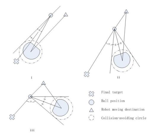
The GOTO_BEHIND state is subdivided into three main situations due to the relative position of the ball, robot and the target. Several veriables are defined to demostrate these relative positions.Let

$$\theta = \arcsin(\frac{r}{|\overrightarrow{m}|})$$

$$\alpha = \pi - \langle \overrightarrow{n}, \overrightarrow{m} \rangle - \theta$$

Where,

$\overrightarrow{m}$ is the collision-avoiding radium $\overrightarrow{m}$ is the vector from robot to the ball $\overrightarrow{n}$ is the vector from the ball to the target

If the robot is in the way between ball and the target ($\alpha \leq \frac{\pi}{12}$, figure i), it moves on the line with constant distance to the ball position to avoid blocking the ball. Then if the robot is on the side of the robot (figure ii,iii), it should go behind the ball to get a proper position to push it to the target. The distance d to the ball has a relation with $\alpha$; the smaller is the closer robot should approach to the ball. So we got

$$d_0 = \begin{cases} \frac{r}{\sin \alpha}, & (\frac{\pi}{12} \le \alpha \le \frac{\pi}{2}) \ r + 5, & (\alpha \ge \frac{\pi}{2}) \end{cases}$$

$$d = d_0 - K \cdot \cos \beta$$

Where,

r is the collision-avoiding radius.

K = d⁰ + dribbleballdist

β is the angle between −→n and −→m, also can be expressed <−→m, −→n >

Potential Based Pass and Receive Searching Potential Based Pass and Receive Searching We have functions to find the best assist point, shoot point or receive point. Several evaluation functions are applied to calculate the rates of each qualified point on the ground according to a set of parameters between ball and goal. For example, we establish a evaluate function E to produce a best assistant point (receive the ball and shoot the goal). All these factors are taken into consideration to evaluate a certain position P:

E(P) = w0 · calShootEval() + w1 · calRobotAdjustEval()
    + w2 · calT oT argetAdjustEval() + w3 · calAwayF romEnemyEval() (2)
   Where,
w[ ] is the weight of each factor
calShootEval() is the possible shoot range at P
calRobotAdjustEval() is the cost for dribbler to adjust to proper angle to
   pass
calToTargetAdjustEval() is the cost for receiver to get to position P with
   proper angle
calAwayFromEnemyEval() is the threats of some near opponent robots

GPU Accelaration For enhancing the processing speed of the algorithm with a tremendous points and saving the CPU computing resources, we use the NVIDIA's CUDA architecture for parallel computing. For example, in the calculation of the shooting point, the court is divided into 400 * 600 units. Each unit calculates a potential energy value taking the shooting angle, passing safety degree, empty area and other factors into consideration. The point gets the extreme low potential energy is regarded as the best destination the shooter should move to.

5 Conclusion

Owing to our all team member hard work, we can obtain this result. If the above information is useful to some new participating teams, or can contribute to the small size league community, we will be very honor. We are also looking forward to share experiences with other great teams around the world.

References

1. Yonghai Wu, Penghui Yin and Rong Xiong, ZJUNlict Team Description Paper for RoboCup2011
2. Yonghai Wu, Penghui Yin, Yue Zhao and Yichao Mao, Rong Xiong, ZJUNlict Team Description Paper for RoboCup2012
3. Brett Browning, James Bruce, Michael Bowling and Manuela Veloso, STP: Skills, tactics and plays for multi-robot control in adversarial environments
4. Yonghai Wu, Xingzhong Qiu, Guo Yu, Jianjun Chen and Xuqing Rie: Extended TDP of ZjuNlict 2009 Robocup 2009
5. Sheng Yu, Yonghai Wu. Motion prediction in a high-speed, dynamic environment.
6. Sebastian Thrun, Wolfram Burgard, Dieter Fox, Probabilistic Robotics, The MIT Press