ER-Force Team Description Paper for RoboCup 2013

Markus Hoffmann, Markus Lieret, Simon Kerschbaum, Michael Eischer, Philipp Nordhus, Adrian Hauck

Robotics Erlangen e.V. Pattern Recognition Lab, Department of Computer Science University of Erlangen-Nuremberg Martensstr. 3, 91058 Erlangen, Germany

http://www.robotics-erlangen.de/

Abstract This paper presents an overview description of ER-Force, the RoboCup Small Size League team from Erlangen located at Friedrich-Alexander-University of Erlangen-Nuremberg, Germany. New developed parts in the hardware and electronic design are described. We will proceed with the control system model. The last paragraph is about the new concept behind our strategy. Furthermore, upcoming changes and improvements are outlined.

Introduction

For this years RoboCup we are improving on all essentials parts of our system. Starting with mechanical aspects, we describe the correct utilization of inductors, our results in finding a robot-model for the control system and ending with the description of the 2013 strategy structure.

Mechanics

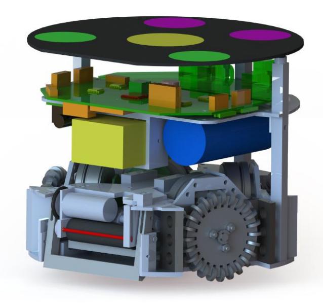
The 2013's Mechanical System will be based on last year's hardware. While main parts are taken over efforts have been made to improve features and eliminate weaknesses. In the following a detailed analysis of last year's system will be given in order to support other teams avoiding design errors.

The focus will be on the kicker, chip kick and dribbler subsystems. Note that the current design showed satisfying performance results as long as it was wellmaintained. But dirt such as fibres of the field carpet influenced this as much as wear and stresses, for example resulting of collisions with other robots. It's the dedicated goal for next year's system to reduce these influences as much as possible to obtain a more stable system that shows a reliable, constant and satisfying performance.

Kicking systems

The kicking systems central unit is mounted in the center of the robot. It consists of an bulky steel housing that accommodates two coils for kick and chip kick. It also reduces influences on the electrical components due to electromagnetic fields.

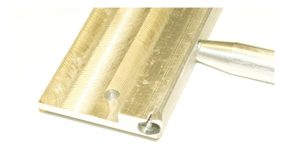
Flat kicker The flat kick has a divided plunger rod: while the front part is made of a aluminum alloy the rear part is made of a ferromagnetic steel. The plunger is attached to the kicking plate which is mounted in a linear slide by two dowels which also limit the flat kicker's movement range. A 6061 aluminum alloy turned out to be not strong enough to withstand the forces that occur when a kick is triggered without hitting the ball. In this case the whole energy has to be absorbed by the slides over the dowels. The remaining wall thickness was not sufficiently high and therefore the holes slackened. Changing the kicking plate material to S235 solved this problem though the price was a decreased maximum ball speed due to the ferromagnetic material and the increased weight of the subassembly. The maximum impuls is given to the ball when the weights of ball and plunger are equal. For this year's robots the material has been changed to 7075 aluminum alloy to gain a maximum ball speed of approximately 8 m/s.

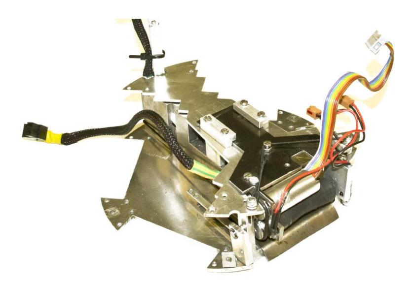
Chip kicker The chip kick was designed last and had to be fit in the remaining space. The extensive dribbler damping plate limited the maximum height of the kicking system and the wheel housings reduced this space further. These constraints made it very difficult to find a satisfying chip kick design. Several parts are redirecting the force exerted by the rear coil. Because of elastic behavior, losses due to angles in joints and friction the initially sufficiently high power is reduced so much that the chip kick can only overcome a distance of approximately one meter.

To improve the chip kick process a motion study has been conducted using a high speed camera. It turned out that due to elastic behavior of the used materials the plate swung back after the first impact on the ball so that energy couldn't be transfered to the ball furthermore. Adding a steel sheet of a thickness of 1 mm that hits the ball instead of the rigid plate improved performance noteable as it acts like a spring and prevents the plate from swinging back.

Dibbler

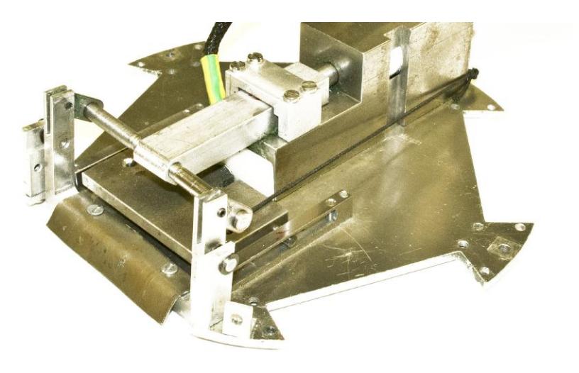
As dribbling motor a Maxon EC16 max motor with 5 Watts is used. The torque is transmitted to the rubber-covered dribbling bar by an O-Ring running in two pulleys. Motor and the dribbling bar are mounted on a linear sliding plate and are placed between the two chip kick handles. The assembly is damped by an elastic band to dissipate kinetic energy of the ball upon receiving a pass and to ensure a maximum of ball handling. However the current dribbling device has two weak spots that lead to inefficiency and high maintenance requirements. First of all the torque transmission is quite loosy. It is intended to replace the pulleys with gears or a bonding of pulley and motor respectively dribbler arbor.

Further changes will improve accuracy in ball position to ensure repeatable shot performance. The damping system will be based on a rotary mount instead to allow more space for other subsystems.

2014's mechanical system

For 2014's RoboCup a new system will be designed. Further enhancements that cannot be implemented in the current system due to lack of space and the extensive dribbler damping system will become available.

The following features are intended to be realized:

• To reduce backlash, the number of functional surfaces and friction losses it is intended to overthink the use of a combination of steel, aluminum alloy and POM or PA 12. Due to POM's low coefficient of friction this material is used for bearings in a pairing with stainless steel.
• Due to the massive loss of power in the current system the next chip kick will be rather a push than a pull mechanism.
• The current linear sliding dribbling device will be replaced with a combination of radial and linear bearing to save space and increase the damping coefficient.

Electronics

Since 2012 we have chosen a new design-concept for our printed circuit boards: every elementary function of the robot is placed on an own board. Subsequent we will explain two of our latest developments. First, we describe the RF-Board, particular the antennas which are already in use. Second, we discuss the Kicker-Board which is currently under development and hopefully finished for RoboCup 2013.

RF-Board

The radio transmission board is placed directly on the top of the robot since 2012. We merged this board with the covering plate and the colored markers of the robot. To optimally utilize the exposed position we integrated the antennas into this PCB. These antennas are etched into the copper-layer of the board.

Fortunately Texas Instruments provides a Antenna Selection Quick Guide [2] for PCB-Antennas and proper footprints. As we use 2.48Ghz as center frequency and a bandwidth of 2MHz we chose the design CC2430DB. This is an Inverted F Antenna (IFA) for 2.4GHz with a bandwidth of 280MHz.

The expected max. gain is +3.3dB with a dimension of 26x8mm on only one copper-layer. The radiated power is almost consistent over the XY plane which means to us the playground. So the radiation angle of the CC2430DB is nearly 360◦ , apparent from Fig. 5. For that reason the relative rotation of the robot to the PC-Transmitter doesn't degrade the signal quality of a transmission.

Before these PCB-Antennas we had ready-to-use RF-modules on duty. These modules had a chip-antenna soldered on the top of the PCB. With this one the transmission quality was very weak and did not satisfy our demands. Altogether we are now very contented with the performance of this antenna. The characteristic of this design allows us to receive and decode a signal even if it had passed three massive brick-walls. This is the performance we need for a RoboCup.

Kicker-Board

Throughout the last years we already designed two of these Kicker-Boards. Unfortunately the version of 2011 had thermal issues like melting and the 2012 release breaks down if the time between turning-off-charging and shooting is too short. This is why we decided to design a new board for this years RoboCup. Below we will outline the circuits and focus on the inductive components. They are more interesting because on one hand they are responsible for the energy throughput and on the other hand they can reduce unwanted current ripple. Also we will present some easy to use formula to calculate suitable values.

Boost-Converter The development of this PCB is still in progress, but the essential high-voltage generation is already tested and is working. We decided to use the boost technology for charging. To control the MOSFET and sense the output voltage the IC LT3757 from Linear Technologie is used. This is a Boost, Flyback, SEPIC and Inverting Controller on one chip [3]. As external components are only a few resistors, capacitors, a coil and a power MOSFET needed. For selecting the best possible coil, we first need to calculate the duty cycle dDC afterwards the inductance of a suitable part.

$$d_{\rm DC} = 1 - \frac{U_{\rm in}}{U_{\rm out}} \tag{1}$$

$$L_{\text{Boost}} = \frac{U_{\text{out}} \cdot d_{\text{DC}} \cdot (1 - d_{\text{DC}})}{I_{\text{out}} \cdot f \cdot r}$$ (2)

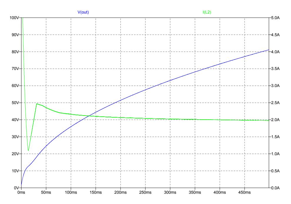
The constant r is the ripple-current-ratio in the coil [4, Page 493]. This should be as small as possible, that's the reason why we used 0.4 for our design, otherwise the coil needs to much place on the board. All other parameters are given through the application. With our data LBoost is calculated to 228µH. To verify these results, we build a small simulation in LTspive IV. The schematic looks like Fig. 6.

There is one more technology for charging the kicker-capacitor which could be suitable for our application: the single ended primary inductance converter (SEPIC). This is a combination of a boost- and buck-converter.

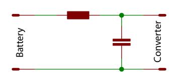
One big advantage of the SEPIC is, that the output is separated via a capacitor from the input, shown in Fig. 8. As a result this high-pass-filter enables the SEPIC to be completely turned off. This is very useful in applications where the output voltage is higher than the input voltage [5]. If we have enough free time until the RoboCup, we will also test the performance of this circuit.

Input filter Another aspect we focused on this year are electromagnetic troubles. So our target is to get a fast charging circuit with minimal EMC trouble. Inside the boost circuit you can't really slow down the flow of the current in order to reduce the electromagnetic emission, because this is essential for the functionality. For that reason the supply line is the biggest problem which can be improved. For high frequencies, as the switching frequency of the boost-converter, the supply line behaves like an antenna. To reduce this effect a input filter is necessary. The value of a suitable inductivity of this filter can be calculated with the following equation.

$$L_{\text{Input}} = \frac{R_{\text{ESR}} \cdot d_{\text{DC}} \cdot (1 - d_{\text{DC}})}{f \cdot (\frac{\triangle I_{\text{in}}}{\triangle I_{\text{PP}}})}$$ (3)

Where 4Iin is the max. acceptable ripple current, RESR is the series resistance of the used capacitor and dDC is the duty cycle of the switching power supply [4, Page 490-492]. The capacity of the input filter Cin should be as big as possible with a low RESR value. For us LInput = 3.8µH and Cin = 470µF works fine for a battery voltage of 16V and a charging power of approximately 30W.

Rework of Velocity Control

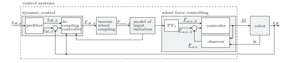
For RoboCup 2013 we made a complete rework of our velocity control. This means – in short terms – we created a detailed mathematical model of the robot and developed a controlling structure that is separated in the two parts observerbased control of the wheel forces and the decoupling control of the velocities. The controlling structures are based on two degrees of freedom state controllers and also take respect of the limitation of the control signals.

In the following text the main aspects of the new controlling approach shall be summarized. The detailed modeling process and the resulting controlling structures can be found in [6].

Rework of the Robot Model

Implementing the existing controlling structures showed that our model was incorrect. For that reason we now wanted to create a very detailed model of the robot that describes all relevant aspects for the movement of the robot.

Since there is a currency control implemented for every motor, which can be seen as a motor torque control, we start the description of the robot with creating a model for the omniwheels. Taking respect of conventional description methods for wheels as well as the special construction leads to a nonlinear description of the wheel forces:

$$F_{wx,i} = \sqrt{(\mu F_{z,\text{ges},i})^2 - F_{wy,i}^2} \cdot \sin\left(C \arctan\left(\frac{B}{\mu}v_{Lx,i}\right)\right)$$

$$F_{wy,i} = F_{z,\text{ges},i} \ \mu_{\text{ow}} \frac{2}{\pi} \arctan(kv_{Ly,i}),$$ (4)

with

$$v_{Lx,i} = -v_{mx,i} + v_{u,i}, v_{Ly,i} = v_{my,i}.$$ (5)

These equations describe the development of the forces Fwx,i and Fwy,i that are transmitted onto the ground in longitudinal direction and cross direction by wheel i. Fz,ges,i is the total force that appears onto the wheel in the direction of the vertical axis. The slips vLx,i and vLy,i are equated by the speeds of the wheel centers vmx,i, vmy,i and the peripheral speed of the wheel vu,i. The wheel center speeds and the peripheral wheel speeds can be evaluated by the robot speeds vx, vy and Ψ˙ and the rotational wheel speeds ω. The combination with the dynamic behavior of the wheels

$$\dot{\omega}i = \frac{1}{J_r} (M_i - F{wx,i}r), \qquad i = 1 \dots 4.$$ (6)

creates a nonlinear state space model for the dynamic behavior of the wheel forces. In this equation, M^i describes the Torque that is created by the motor at the wheel and can be seen as the input signal of the system.

The second step in describing the robot is to transform the wheel forces onto the robot assembly so that the dynamic behavior of the robot can be described in the last step. In this step we also took respect of the fact that the center of mass is not located in the ground plane but can be found in a constant height h. For that reason accelerating the robot leads to a different distribution of the weight of the robot onto the different wheels.

To summarize the results of the modeling process, we get two static matrices that allow us to transform the wheel forces into assembly-based horizontal forces and equate the change of the vertical forces onto the wheels:

$$\underline{F}{H} = \underline{\underline{G}}{x}\underline{F}{wx} + \underline{\underline{G}}{y}\underline{F}{wy} = \underline{\underline{G}}\ \underline{F}{w},\tag{7}$$

where $\underline{F}_H = \begin{bmatrix} F_x \ F_y \ M_z \end{bmatrix}$ describes the overall forces in x- and y-direction and the overall torque related to the vertical axis of the robot. In addition:

$$\underline{F}{z,\text{ges}} = \underline{F}{z,0} + \underline{F}{z} = \begin{bmatrix} F{z0,1} \ F_{z0,2} \ F_{z0,3} \ F_{z0,4} \end{bmatrix} + \begin{bmatrix} F_{z,1} \ F_{z,2} \ F_{z,3} \ F_{z,4} \end{bmatrix} = \underline{F}{z,0} + \underline{\underline{G}}{M} \begin{bmatrix} 0 & h & 0 \ -h & 0 & 0 \end{bmatrix} \underline{\underline{G}} \underline{F}_{w},$$ (8)

where $\underline{F}_{z,0}$ are the forces in vertical direction that appear initially on the wheels and $\underline{F}_z$ are the changes of those forces caused by wheel forces $\underline{F}_w$ .

The third part of the modeling process is the description of the dynamic behavior of the robot. In that turn we also regarded the fact that the center of mass might not be located at the geometrical center of the robot. Analyzing the kinetic and kinematic relations at the robot lead to a nonlinear coupled state space system:

$$\underbrace{\begin{bmatrix} \dot{v}_x \ \dot{v}y \ \dot{\underline{\Psi}} \end{bmatrix}}{\underline{\dot{v}}H} = \underbrace{\begin{bmatrix} v_y \dot{\underline{\Psi}} \ -v_x \dot{\underline{\Psi}} - l_s \dot{\underline{\Psi}}^2 \end{bmatrix}}{\underline{\underline{f}}(\underline{v}H)} + \underbrace{\begin{bmatrix} \frac{1}{m} + \frac{l_s^2}{J_z} & 0 & -\frac{l_s}{J_z} \ 0 & \frac{1}{m} & 0 \ -\frac{l_s}{J_z} & 0 & \frac{1}{J_z} \end{bmatrix}}{\underline{\underline{E}}H} \underbrace{\begin{bmatrix} F_x \ F_y \ M_z \end{bmatrix}}{\underline{\underline{F}}_H}. \tag{9}$$

The vector $\underline{v}_H$ contains the velocities of the robot in x- and y-direction as well as its rotational speed. It is very interesting to see that there is a coupling between the input signals (robot forces $\underline{F}_H$ ) and the robot states ( $\underline{v}_H$ ) as well as between the states among themselves.

Rework of the Velocity Control

For controlling the velocities of the robot we use the structure that can be seen in Fig. 10. Explaining the single parts in detail would lead too far at this point.

The important things are:

• decoupling controller and controller for wheel forces contain integrator part
• the prefilter creates trajectories for the velocities that take respect of the limited wheel forces and thus can be realized by the robot
• the model of the input limitation ensures that the wheels do not slide over the ground and prevents windup of the velocity controller
• the wheel force observer estimates the transmitted wheel forces using the measured wheel speeds and the motor torques

The simulation of the found structures lead to very good results in the dynamic of the robot. For implementing the controlling structures on the real systems we try to install the components step by step but the immense amount of parameters that need to be identified hardens that work amongst others.

Strategy

During last years robocup we were able to learn quite much about the pros and cons of our strategy design. Like the Skill-Tactics-Play design, our strategy had three layers. However having chosen to let the plays control the tactics quite directly, much of the task logic was moved into each play. The design proved sufficient for simple reactive behaviour, but it turned out to be nearly impossible to implement a passing sequence or other advanced behaviour. In addition we opted for stateless tactics, which offer the benefit of (nearly) never getting stuck. But it also complicated the implementation of tasks like catching the ball or shooting a goal, as these require hysteresis for good performance.

We did a full redesign of our strategy which now is loosely based on STP. As an important difference to STP, the play layer is complemented with so called robot pools that implement a default behaviour for every robot.

Plays

In our design a play just performs a fixed action sequence to manipulate the ball like passing or passing and shooting a goal. A play uses a subset of our robots that is chosen when the play is started and then remains unchanged during play execution. In difference to STP, we don't use an opportunistic reassignment of robots. Instead, that behaviour is implemented by choosing and replacing plays based on their success probability. Like several other teams, we implement our plays using state machines [7] [8].

A robot pool is a group of robots that defends our goal or assists the attacker. Every robot belongs to one of these groups. For robots that are controlled by a play this default behaviour is suppressed. That way a play only has to control robots relevant for its current action, simplifying the implemenation of a play. Robots that are no longer controlled by a play return immediately to their default behaviour. This allows us to have the keeper start a pass sequence and then return to defending.

A play selects its robots from the pools that match the intended behaviour of that pool. A freekick for example will be performed by a robot from the attacker assistant pool. Thus the pools provide us with the ability to easily control our strategy aggressivity by changing the number of robots assigned to the assistant or defense pools. We intend to implement this behaviour based on metrics like which team owns the ball, where it is moving etc. In order to have a stable behaviour we added a hysteresis on the number of robots that delays moving robots between the pools.

Play selection

In each frame our plays are grouped, based on their success probability, which can be one of the following values: no (will never succeed), unlikely, may succeed, very likely and forced by referee. By default, a play that could be excecuted "may succeed". Only plays that provide opportunistic behaviour are "very likely" to succeed.

To select a play we use weighted random selection from the group with the highest probability. When there's already an active play, it is only replaced, if the new play belongs to a group with higher success probability, than the active one is currently in. Using that mechanism opportunistic behaviour is yielded by play replacement. It also offers play termination for free, as a play that has finished is now in the group "no" and will be replaced by any applicable play.

Conclusion

Changes in kicking plate material, reduction of EMC-troubles, rework of the Robot-Model and a strategic redesign throughout robot pools will hopefully show up new perspectives for RoboCup 2013.

References

1. Andersen, A.: 2.4 GHz Inverted F Antenna. Technical report, Texas Instruments (2008)
2. Texas Instruments: Antenna Selection Quick Guide (2013)
3. Linear Technology: LT3757/LT3757A – Boost, Flyback, SEPIC and Inverting Controller (2008)
4. Brander, T., Gerfer, A., Rall, B., Zenkner, H.: Trilogie der induktiven Bauelemente. Swiridoff (2008)
5. Dostal, F., Sclocchi, M.: Die Vor- und Nachteile der Power-Managment-Topologie SEPIC. http://www.elektronikpraxis.vogel.de/stromversorgung/articles/174511/
6. Kerschbaum, S.: Modellbildung und Reglerentwurf für die Horizontalbewegung eines Roboters mit omnidirektionalem Antrieb. Bachelor's thesis, Friedrich-Alexander-Universität Erlangen-Nürnberg (2013)
7. Adhami-Mirhosseini, A., Babersad, O.B., Jamaati-tafti, H., Asadi-Dastjerdi, S., ziyadloo, S., Ganjali-Poudeh, A.: MRL Extended Team Description 2012 (2012)
8. Wu, Y., Yin, P., Zhao, Y., Mao, Y., Wang, Q., Xiong, R.: ZJUNlict Extended TDP for RoboCup 2012 (2012)