KIKS 2013 Extended Team Description

Ryu Goto, Takaya Asakura, Naomichi Fujii, Kosuke Matsuoka, Masataka Mizuno, Tetsuya Sano, Yuya Onuma, Hiroshi Nagata, Masato Watanabe, Toko Sugiura

Toyota National College of Technology, Department of Electrical and Electronic engineering, 2-1 Eisei-cho, Toyota Aichi, 471-8525, Japan

http://www.ee.toyota-ct.ac.jp/~sugi/RoboCup.html

Abstract This paper presents a detailed description of KIKS in addition to the team description paper of small size league in RoboCup 2013. Our robots and systems are designed under the SSL 2013 rules in order to participate in the RoboCup competition. The major improvements in this year are the enhancement of the performance and robustness of wheels, electrical circuit and automatic control system. The overviews of them are described

1. Introduction

In RoboCup world competition, our team has continuously participated since 2004. We came in top 4 in Singapore, Istanbul and in top 3 in Mexico last year. Since we are aiming for higher place compared with last year, further improvements have been done in this year.

One of the educations for creative minds of students is using the robot contest. We have executed the robot contest in our college just like RoboCup junior every year. So, main purpose of our participation to the RoboCup world competition is confirmation and evaluation of effect for creativity.

In last year, there was a problem that the travelling performance of robots was poor. So, we redesigned a new wheel and improved the stability of the robots under travelling on the field. We also redesigned speed controller on the AI server. As the results, response performance was better than that of last year.

The main topics of robot's hardware developed for 2013 model are following terms:

Improvement of the wheels
Improvement of the electric circuit
Improvement of the speed controller on the AI system

2. Hardware of the robot

In 2013 model, we redesigned focusing on the following points:

Lighter body
Lower center of gravity
Improvement of layout of wheels
Simpler mechanism and maintenance

The new robot is shown in Fig. 1 with previous robot. The specification of a robot is summarized in Table 1.

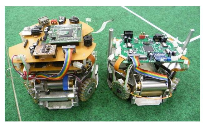
Fig. 1 Comparison between New model (right side) and previous model

Table 1 Specification of a robot

	2012 version	2013 version
weight	2.4kg	1.9kg
Main material	Aluminum alloy
Driving motor	maxon EC45flat(30watt)
Gear ratio	3.6:1	4.0:1
Wheel diameter	56mm	50mm
Number of solenoids	Straight kick:1(round) Chip kick:2(round)	Straight kick:1(flat) Chip kick:1(flat)
Straight kick power	Ball speed of 8m/s (max 10m/s)	(max 9m/s)
Chip kick power	3.0m away from robot with initial angle of 40°

2.1. About the lighter body

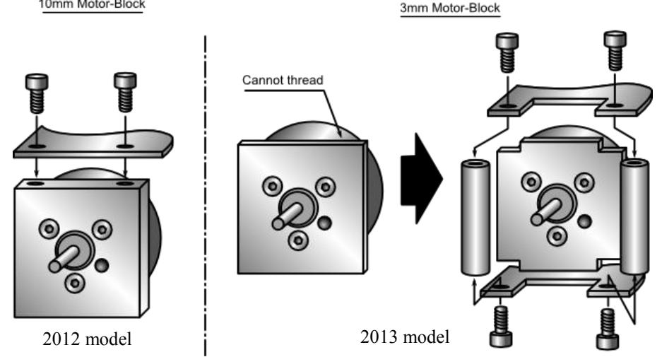
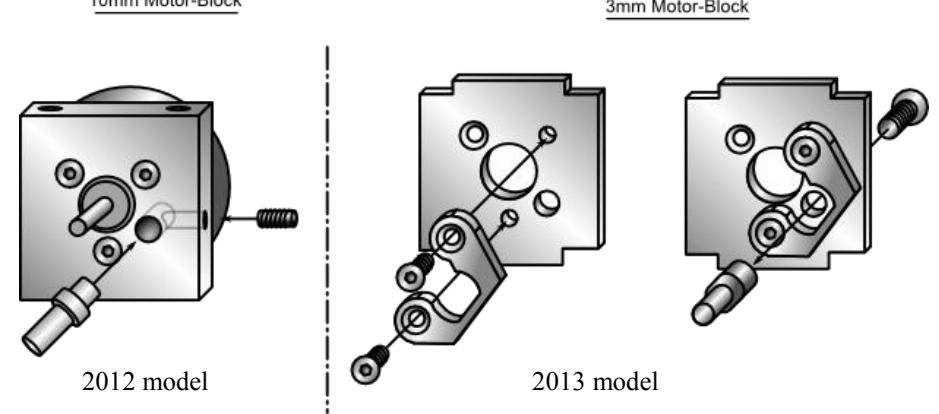
For the reduction of weight, Aluminum thicknesses of each part are reduced as shown in Table 2. The method to fix the motor-block and the motor-shaft for 2013 model are shown in right side of Fig. 2 and Fig. 3, respectively.

Table 2 Thickness of each part

	2012 model	2013 model
Chassis	5mm	3mm
Motor-block	10mm	3mm

Fig. 2 Improvement of method to fix motor-block on the body. Left one shows the previous model.

Fig. 3 Improvement of method to fix motor-shaft on the block. Left one shows the previous model.

2.2. About the lower center of gravity

To decrease the center of gravity of robot, we improved by using the shorter diameter wheels and flatten solenoid.

2.2.1. Improvement of wheel

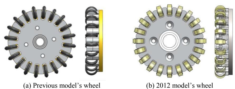
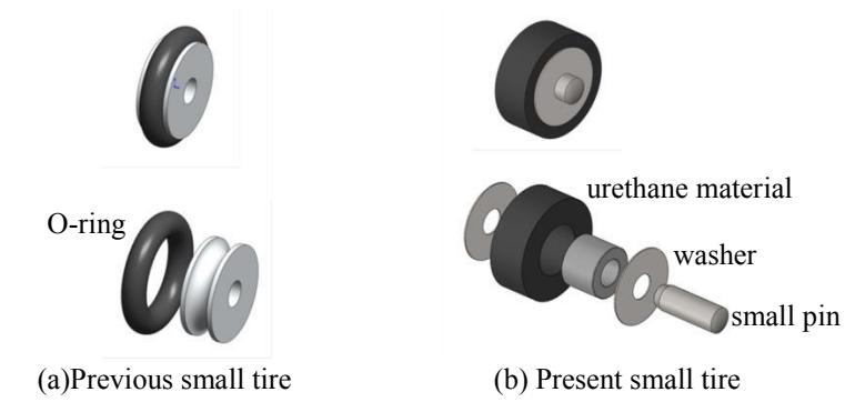
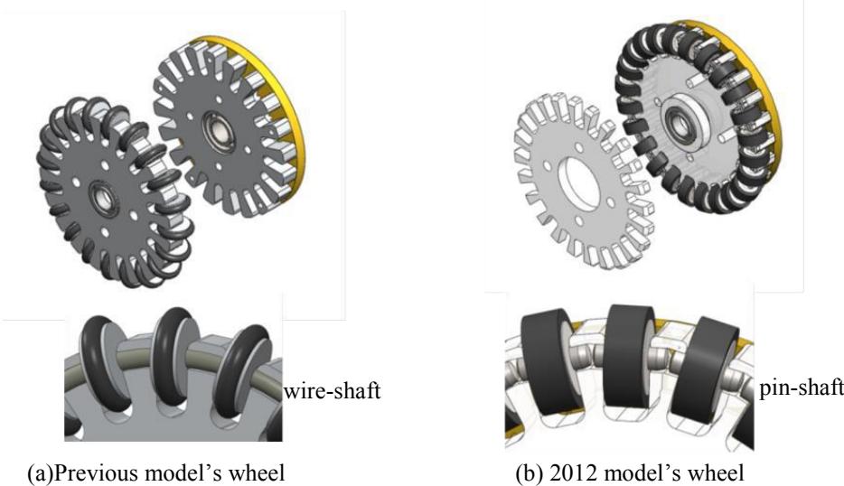
Since 2011 competition, we have used the same brushless motors as many teams do. But, there was a problem in previous wheel for performance of straight-running stability of the robot. That is, our robots were not able to run straight stably under the condition of max speed of 2ms$^{-1}$ and acceleration of 3ms$^{-2}$. Figure 2(a) shows the previous wheel. There were two reasons why straight-running stability was bad. One was that the small tires on wheel do not rotate smoothly. There were frictions between small tire and the tire's house. Another one was that the characteristic of friction to the playing field for rubber small tire is not so good. It is made to occur the slipping of robot in play, because of use of O-rings with cross-section of circle with smaller ground contact area. Thus, we redesigned new wheel to solve these problems. It was changed to new design for the small tire as shown in Fig. 4(b).

2.2.2. Shorter radius of wheel

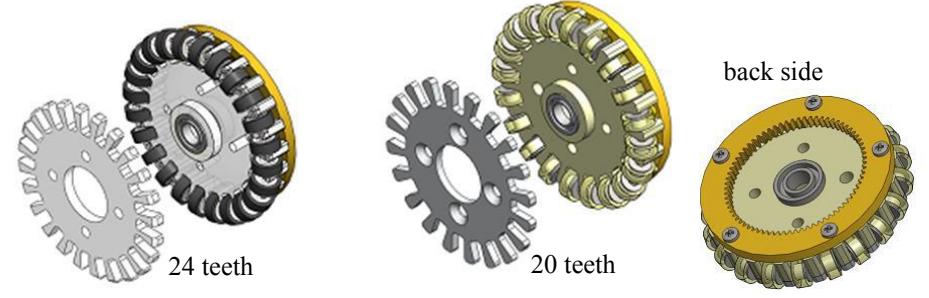
In fact of RoboCup 2012, it was used the wheel as shown in Fig. 7. That is, the number of small tire is decreased to 20 from 24 and the front plate was changed from resin to duralumin in order to enhance the strength of the wheel itself. In addition, the material of the small tire was changed to MC nylon from polycarbonate. The performance of 2012 model was better than that of previous one. But it remains some problems. One of the important points is wheel size. It is too long because it designed to fit the shaft of previous wheel. Another one is too bad for the precision of the shaft itself.

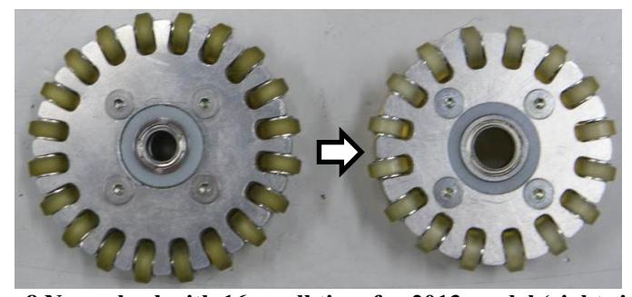
So, in 2013model, it is short for the diameter of wheel from 56mm to 50mm. It is effective for lower center of gravity, lighter weight and decreasing of the wheel's moment of inertia. Simultaneously, the number of small tires is decreased to 16 from 20. The photo image of new wheel is compared with that of 2012 model as shown in Fig. 8.

Fig. 7 Wheel actually used in RoboCup 2012 (right one). Left one with 24 small tires is for the test.

Fig. 8 New wheel with 16 small tires for 2013 model (right side)

2.2.3. Flattened solenoid

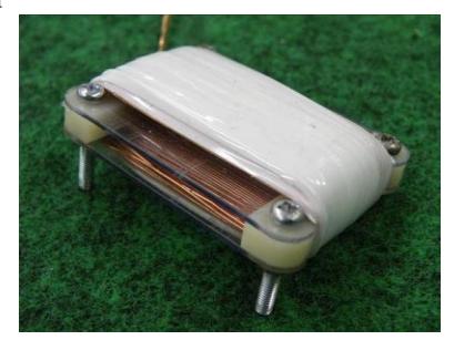
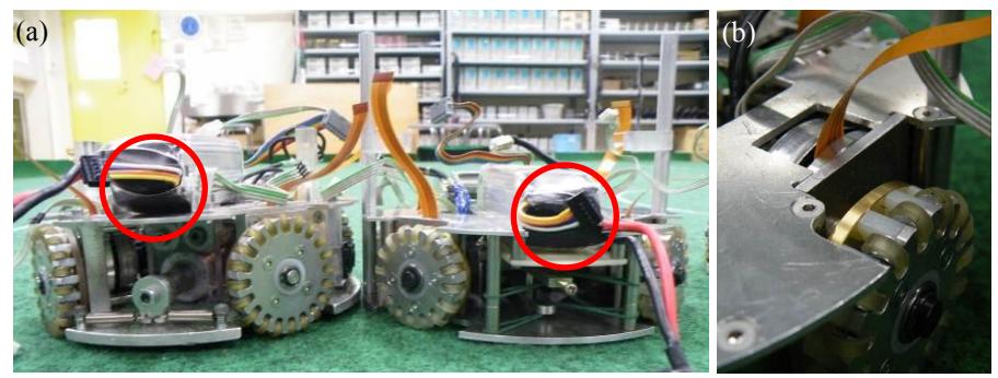
We have used conventional round-shaped solenoids until 2012. In 2013, we developed flatten solenoids. Its performance is same as the previous one. The image of new solenoid is shown in Fig. 9. We could use same parts for both solenoids of chip kick and straight kick. Moreover, the top of motor is mostly located above on the metal plate. As the results, the height of robot and position of battery, that is, the center of gravity is lower than 2012 model as shown in Fig. 10.

Fig. 10 (a) Lower height of new robot (right one; red circle shows the battery, left one is previous model) and (b) top of the motor for driving wheel.

2.3. Improvement of wheels-layout

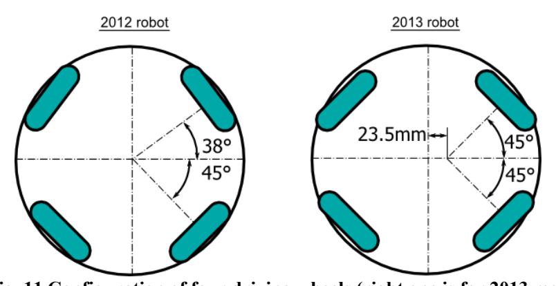
We improved the configuration of four driving wheels as shown in Fig. 11 by decreasing of the diameter of wheel. By placing all the wheels 45 degrees, the running speed of robot for omni-direction was made mostly equal and the easy control was achieved.

Fig. 11 Configuration of four driving wheels (right one is for 2013 model)

2.4. Simplification for mechanism and manufacturing

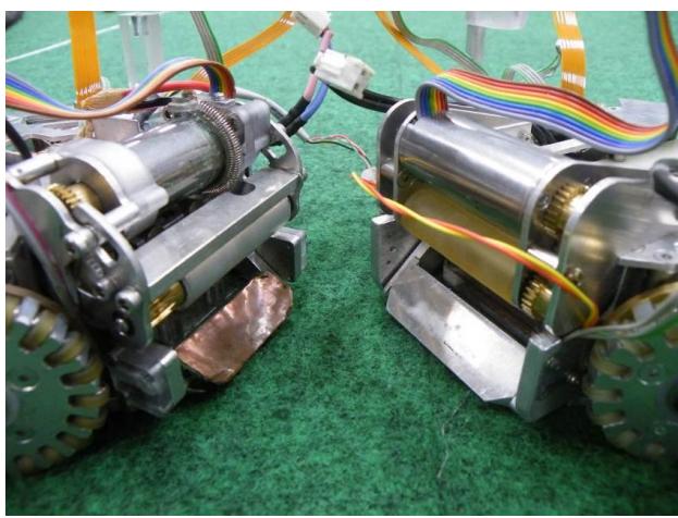
It is important to make robot easily because we have no enough members and time to develop and manufacture. The rotation-bar of dribbling device of 2012 model was movable for up- and down-ward, but in 2013 robots it was fixed as shown in Fig. 12. Thus, we could realize easily making and decreasing of trouble. Furthermore, the number of parts is decreased, and a lot of ready-made parts are used.

Fig. 12 New dribbling device in 2013 model (right side)

3. Electrical design

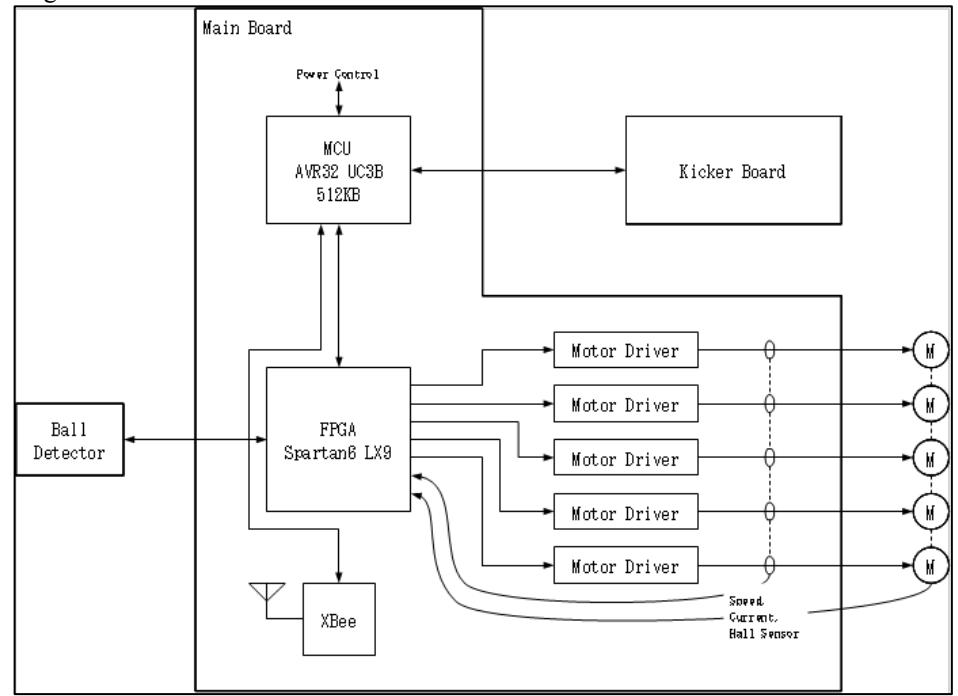
In this year, we have redesigned our electrical circuits. First, we introduced the FPGA board (Xilinx XC6SLX9). FPGA circuit controls all five motors mounted in a robot. That makes it possible to reduce the size of electronic circuit. Second, we replaced the previous discrete driver circuit with the IC (TI DRV8332) for motor-driver circuit. This integrated motor-driver chip has three half bridges and gate drivers, an over-current protection and an over-temperature protection. It is expected that the electric trouble will be decrease for the motor driver circuit. Figure 13 shows the block diagram of electronic circuit.

Fig. 13 Block diagram of electronic circuit

3.1. Motor Driver

Five motor-driver ICs (DRV8332) are mounted on the main board. Four of them are for the travelling wheels and one is for the dribbling device. The current for each four travelling-wheels is monitored by two IC (TI INA213), and is used for current restriction. Each motor has hall sensor, and each wheel's motor has an optical encoder (E4P). These signals connected all to the FPGA. The openMSP430 core of 16bit processor (running at 45MHz) calculates the control parameters based on above signals by period with 2ms in FPGA board.

3.2. Kicker

Our robots have two capacitors (each 250V 1500uF) connected at parallel. They are charged up to 240V by boost converter of DC circuit. Two solenoids for straight-kick and chip-kick are operated by two IGBT devices. For charging to the battery and the control of kicking device, they are performed by a micro-computer (Atmel ATXMEGA32A4U). The UART is used for the communication between kicking- and main-board with speed of 250kbaud.

3.3. Ball detector

The ball is detected by a photo interrupter. The driver (Hamamatsu Photonics S6809) output the signal whether a ball is in front of the robot by using IR LED.

3.4. Microcontroller

We chose an ATMEL AT32UC3B0512 microcontroller as main CPU. It controls the power management of circuit, wireless communication, communication to the FPGA and the kicker board etc., and runs at 60MHz. The firmware was developed to check for the circuit and to communicate to PC through by USB port.

4. Software design

(Section introduction)

4.1. Improvement of Speed Controller

In TDP of this year, we reported improvement of robot's velocity controller. The controller change the degree of decreasing velocity by using internal coefficient, however, it was not able to slow down with the speed taking into account maximum acceleration. Now, we can do that by improving of the function for internal sliding mode controller.

4.2. Previous Controller on TDP

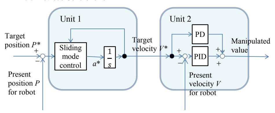
New controller has 2 units as shown in Fig. 14. The Unit 1 outputs the ideal motion speed based on the robot's position with considering of max acceleration and convergence velocity $V^$ to the target position $P^$. We applied tentatively sliding mode control theory for speed of robot. As the result, it can easily control them. The equation of sliding mode parameter $\sigma$ and ideal acceleration $a^*$ are shown as follows:

$$\sigma = H(P^* - P) + V^*$$

$$sign(x) = \begin{cases} 1 & (x > 0) \ -1 & (x < 0) \end{cases}$$

$$a^* = a_{max} sign(\sigma)$$

where H is positive efficiency and used to decide convergence velocity.

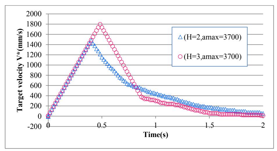
The Unit 2 outputs the manipulated value to follow the robot's velocity V to target velocity $V^$ getting from Unit 1. Since it has two-degree-of freedom control as shown in Fig. 14, it is robust against the disturbance. Fig. 15 shows the dependence of target velocity for parameter H. It is shown that the target velocity $V^$ is varied depending on the coefficient H of eq.(1a). Especially in the case of H=3, it is shown that the target velocity $V^*$ is decreased linearly from the point of slow down. It means that the precipitous change in velocity does not achieve actually. Thus, it is important to choose appropriate parameter to get optimum performance under the condition of stable control loop by applying.

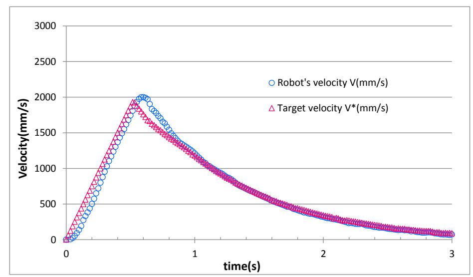
The time dependence of the velocity until arriving to the target position is shown in Fig. 16. It is shown that the agreement between robot's velocity and target velocity is fairly good. That is, it is found that the velocity of robot will be able to respond within 100msec.

Fig. 14 New speed controller with two units

Fig. 15 H dependence of Target velocity V*

Fig. 16 Time dependence of velocity for robot

4.3. New Controller with changeable coefficient

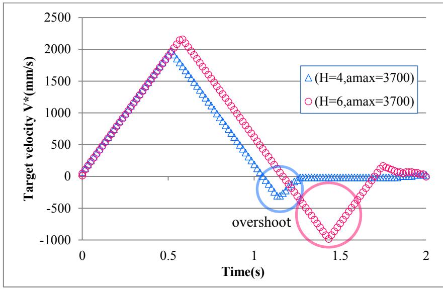
As mentioned above, in new Controller, it is caused an overshoot for target velocity $V^*$ as increasing of parameter H, as shown in Fig. 17.

Thus, we try to use the following equation to solve this problem:

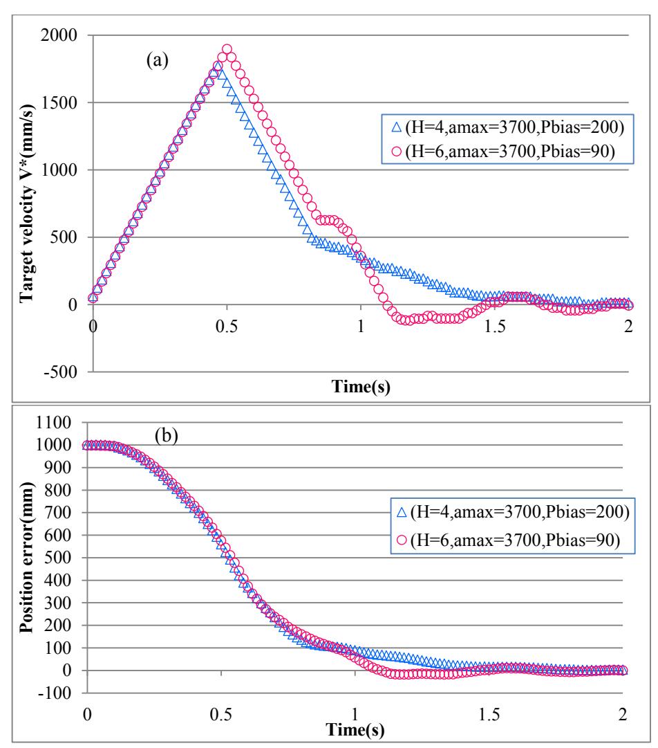
$$\sigma = \begin{cases} (P^* - P + sign(V^)P_{bias}) + \frac{sign(V^)}{2a_{max}}(V^)^2 & (HV^ > a_{max}) \ H(P^* - P) + V^* & (HV^* < a_{max}) \end{cases}$$

This function performs the slowdown of target velocity with constant of acceleration $a_{max}$ and traces that appropriately on the sliding mode. $P_{bias}$ is the constant and used to adjust the region for connecting two functions. As the results, we obtained the performance shown in Fig. 18(a) and (b). In figures, it is same value for the parameter H and $a_{max}$ in Fig. 17. It is found that even if H is big value, the robot can respond to target velocity and the position without remarkable overshoot. Now, we can control the velocity of robot properly if Unit 2 in Fig. 14 will be able to respond sufficiently.

Fig. 17 Overshoot of target velocity depending on the parameter H

Fig. 18 Time dependence of velocity (a) and position error (b) for robot

5. Conclusions

Our robots have been continuously improved in every year. As the results, the travelling performance is getting better and robots are able to move more quickly than last year.

We hope that our robots will perform better in this coming competition.

References

- adfa, p. 3, 2012. © Springer-Verlag Berlin Heidelberg 2012