TIGERS Mannheim
Andre Ryll, Nicolai Ommer, Daniel Andres, Dirk Klostermann, Sebastian Nickel, Felix Pistorius
Department of Information Technology, Department of Mechanical Engineering Baden-Wuerttemberg Cooperative State University, Coblitzallee 1-9, 68163 Mannheim, Germany
Abstract This paper presents a brief technical overview of the main systems of TIGERS Mannheim, a Small Size League (SSL) team intending to participate in RoboCup 2013 in Eindhoven, the Netherlands. This year, we redesigned our bots' mechanic and electronic to improve overall precision and to add new features. Our software showed very reliable and stable, so we could concentrate on some improvements in the artificial intelligence. One main module is a learning play finder that uses a knowledge base to determine a play set for the current situations.
1 Mechanical System
In the last two years our first robot design has shown some serious mechanical problems. To overcome these issues we decided to build a new robot from scratch. The old and the new robot are shown in figure 1. The mechanical specifications are listed in table 1.
The old robot had two main problems. First, we underestimated the power of the kicking device and the forces during a shot. The straight kicker connection from solenoid to plunger was only 3mm in diameter. The thin connection bent regularly and even the threads used in the parts were vaporized to fine aluminum powder after some shots. The dribbling bar had a similar problem. In close contact situations with other robots our dribbling bar bent and made precise dribbling impossible. The second major problem which is not only limited to the mechanical construction was the overall precision of our system.
To improve the mechanical precision we reduced the diameter of the wheels by moving the transversal rollers more inward to the center of the wheel. Furthermore we changed from an external spur gear with a ration of 30 : 100 to an internal spur gear with a ration of 15 : 50. This significantly reduces the height of robots drive unit and thus gives more space for capacitors and electronics. It also moves the mass center down which helps accelerating the robot faster. The position of the encoder changed in the new design, too. The encoders were previously connected to the wheel shaft and are now connected to the motor. This increases their resolution by the gear ratio. Additionally the encoders themselves have a higher tick rate. The old ones made 1440 ticks per round (US Digital, E4P). The new ones make 2048 ticks per round (US Digital, E8P) when sampling every transition in the encoder signal. To mount the encoders to the motor we had to back-extend the motor shaft. This job is easily accomplished when using a arbor press. The modification of the encoder position yields a increase in odometry resolution of factor 4.74.
To resolve the issues with the kicking and dribbling systems, we increased the diameter of the straight kick shaft to 8mm and the dribbling bar to 12mm. The new version of our robot also includes a chip kicker based on the flat shaped solenoid design. Furthermore we changed the top cover which is now made out of two POM parts, whereas the top one has the pattern circles perfectly milled. Thus the pattern should always perfectly align with the front of our robot which also increases our precision.
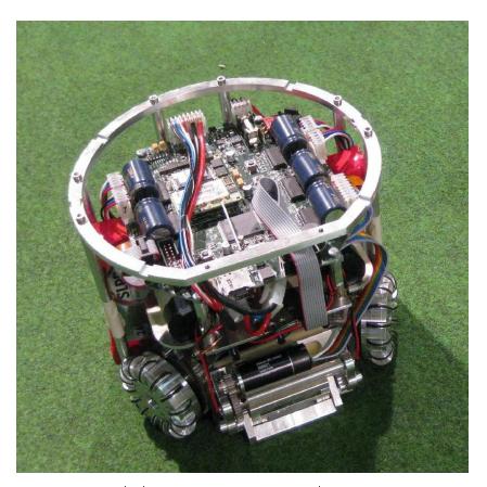
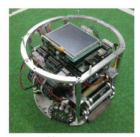
Table 1: Mechanical Specification
| Robot version | 2011/2012 | 2013 |
|---|---|---|
| Dimension | Ø180 x 148mm | Ø178 x 148mm |
| Max. ball coverage | 15.3% | 12.3% |
| Driving motors | Maxon EC-45 at 30W | Maxon EC-45 at 30W |
| Gear | 30 : 100 | 15 : 50 |
| Gear type | External Spur | Internal Spur |
| Wheel diameter | 58mm | 51mm |
| Encoder | US Digital E4P, 1440 PPR | US Digital E8P, 2048 PPR |
| Dribbling motor | Maxon EC-16 15W | Maxon EC-16 30W with |
| planetary gear head | ||
| Dribbling gear | 20 : 40 | 48 : 24 |
| Dribbling bar diameter | Conus 4-8mm | 12mm |
| Chip kicker | No | Yes |
| Straight kicker | Yes | Yes |
2 Electrical System
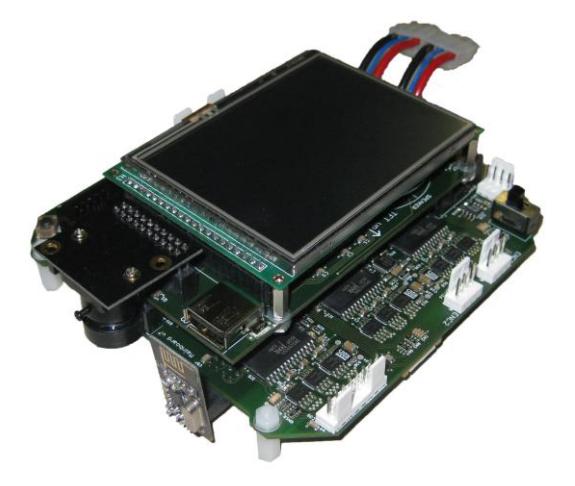
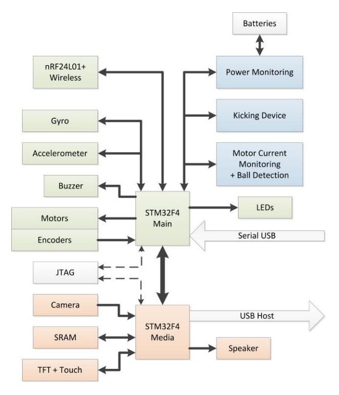
To complete our new robot we also made a new electronics board which is depicted in figure 2. It is actually made of two custom stacked boards with an TFT Display on top. The new board combination (named mainboard and extension board) has several new features. First of all we changed the main processor from a Cortex-M3 with 72Mhz to the next generation of this chip, a Cortex-M4 with 168Mhz (STM32F4). This processor controls among other things the motors and reads encoder signals. Most of the low level motor control is done in hardware interrupt routines and thus only generates minimal processor load. The motor PWM signals use a frequency of 20kHz. The encoder signals are fed directly into some hardware timers which are periodically polled to calculate the current wheel speed.
Connected to the main processor are also an accelerometer and a gyroscope to provide additional sources for the on-board filtering. Minor features include some LEDs for signaling fatal problems and a buzzer to generate an audible signal. Furthermore a USB-to-Serial bridge is connected to the processor to provide a debug interface to the user. The complete system architecture is shown in fig. 3.
Co-Processors
Two on-board ATmegas from Atmel (ATmega168) are connected via SPI to the main processor. One is used to monitor the cell voltages of our batteries (two 2400mAh 2S1P packs) to prevent damage from deep discharge. The other one is used to monitor the motor currents which are differentially measured above a shunt resistor on each motor drive circuit block. It also acts as an AD-Converter (ADC) for the infra-red light barrier in front of the robot. Although the Cortex-M4 has its own ADC built in we chose to use external ATmegas because we can offload digital filtering to them. Additionally there is a lot of digital noise around the main processor.
Kicker
A third ATmega is used on our external kicker board, which is mounted near the bottom of the robot to generate some distance between the very noisy kicker circuit and the sensitive mainboard. The main processor communicates via SPI with all ATmegas. A custom data protocol with checksums ensures the consistency of the exchanged data. The kicker ATmega controls the charging of the capacitors (2x 2200uF/250V) and the discharge through high-voltage IGBTs. During charging it monitors the voltage and the current flowing through the power part. Based on the current voltage a different duty-cycle is selected which decreases the overall charging time. Our current first-try implementation reaches a voltage of 200V in 2s. The current monitoring can be used to detect hardware malfunction or to limit the duty-cycle as well. In contrast to the old design our kicker is now based on the step-up converter principle as this technique requires much less space on the kicker board.
Wireless
Our old robot used DECT modules which had the great advantage of using the 1.9Ghz frequency band which is rarely used in RoboCup. This module is closed-hardware and thus a black-box for us. We encountered a varying latency up to 50ms. These problem made the closed-loop control of the robot quite difficult and inaccurate as we had to deal with a varying dead-time. Furthermore the module has only a throughput of 115.2kBit/s.
Due to all these disadvantages we decided to select another wireless module for our new robot. The nRF24L01+ module from Nordic Semiconductor is wellknown and has proven to work well in the Small Size League. Although it works in the 2.4Ghz range it allows to select from 125 different channels. The upper channels are also forbidden for commercial WLAN equipment, which allows to select a good frequency even if there is a lot of such equipment or other teams using this module. Additionally this module allows data rates of up to 2MBit/s. We built a custom base station for these modules which has a wired network connection. The station electronic is built around a Cortex-M3 from STmicroelectronics connectivity line which allows to interface the network with up to 100MBit/s. The base station uses a time-division protocol to communicate with the bots, thus we only need one channel to communicate with all bots. As this system is totally known and open hardware we shall be able to minimize latency problems.
Extension Board
The extension board on top of the mainboard is equipped with another Cortex-M4 (STM32F4) which is also clocked at 168Mhz. It is connected via a high-speed serial connection to the main processor. It interfaces a 320x240 pixel TFT display with touchscreen capability to provide an easy interface to the user. Compared to buttons on the boards it has the great advantage of being a reconfigurable UI. Furthermore the so called media processor also interfaces 2 MB of external SRAM which is needed for storing and processing images as the Cortex-M4 only has 192kB internal RAM.
The media processor also features an USB Full-Speed Host port. We developed drivers for interfacing USB mass-storage devices and are currently working on support for Human Interface Devices (HID class). Supporting HID devices also allow us e.g. to plug a keyboard into the robot and use it for some kind of text console on the display. Even more sophisticating is the option to plug a wireless gamepad into the host port and control the robot directly with a game pad without the need for any other infrastructure. This is mainly intended for Human-Computer matches or for demonstration events.
Besides these features the media processor also interfaces a digital audio system via an I2S bus. A small speaker is mounted below the display on the extension board. Unlike the buzzer this speaker can play real sounds or music. The audio system has already been successfully tested by playing a WAV file from an USB stick.
On-Board Vision
One of our greatest innovations this year is the usage of an on-board vision module. The OV7725 camera module allows to capture images of 640x480 with a frame rate of 60fps. With a reduced resolution of 320x240 it can even capture 120fps. The images are captured via a DCMI interface which is hardware supported by the Cortex-M4. The media processor can directly store the images in the external SRAM via a DMA transport and thus does not consume CPU cycles when fetching images. The processor can focus on processing the images. Our current setup uses the camera facing down to the dribbling device of the robot. We intend to use it for ball detection if the ball is close to the robot. With this feature we can even see the ball in close-contact situations where the field-cameras cannot identify the ball. By signaling the ball position back to our central software we have an additional information channel for our AI. Furthermore the camera can be used to detect the horizontal position of the ball in front of the robot and also if the ball is bouncing off of our dribbler. This information could be used to improve our dribbling skills.
Control
With a whole processor only used for image processing and the availability of a floating point unit in the Cortex-M4 we plan to move our filtering and control from the main computer to the different robots. The robot has several on-board sensors that can be used for control. These include high-resolution odometry, motor current, accelerometer and a gyroscope.
All these sensors can be combined by a Kalman-Filter and used for a cascading closed-loop controller. The accelerometer and the gyroscope can be polled with up to 400Hz, the motor current and the encoders with up to 200Hz. The global position comes in at 60Hz from the main computer. The Kalman-Filter operates on global coordinates. The control output is fed into a non-linear transformation stage which maps them to local wheel speeds. In return the sensor data is also converted back to global values. To remove the dependency and non-linearity of the X and Y components on the rotation rate, we plan to locally turn our coordinate system on the bot, and thus have three independent state variables.
A simple velocity based control is already implemented and yields a processor usage of approx. 1%. Together with the other tasks the main processor is over 90% idle. The media processor is idle 99% of the time. Additionally STmicroelectronics provides a DSP library for the Cortex-M4 that includes operations for matrix calculations. These operations are already optimized for the floating point unit and the available DSP instructions. Overall there should be sufficient computing power to do an on-board sensor fusion and control. The estimated state and velocity will also be transmitted back to the main computer, to let the AI know where our robots are.
3 Software
The central software, called Sumatra, has proven to be a stable and reliable component with much potential in extensibility. Last year, we focused on basic functionality and reliability to ensure that we are able to play games fluently. This year, we want to extend and optimize certain sub components. We focus on the play strategies of our AI and an enhanced precision with the new robots.
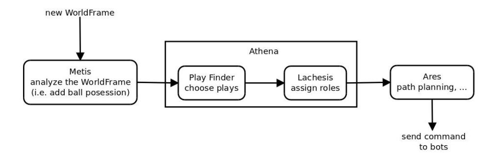
The architecture of Sumatra has not changed compared to last year and can be looked up in the TDP from last year. We are still using a play-role concept where each robot has one role at a time and a play coordinates a set of roles. There are usually at least three plays running at a time for attack, defense and support. Plays will change very frequently. One challenge for RoboCup 2013 is to decide which plays are appropriate in which situation. We developed a play finder with a learning algorithm to learn from certain situations and optimizing the selection of plays. It was initiated in a project of the lecture knowledge based systems.
3.1 Play Finder
The play finder is a sub module within Sumatra that decides about the set of plays for the current situation (see figure 4 for overview of information flow). The former implementation had hard coded decisions that were primarily based on the referee messages. Depending on the referee message and the number of bots, a static set of plays was selected. As there were only few plays available in Sumatra, this had no critical influence to the competition, but it was hard to maintain if new plays had to be integrated.
Therefore a new abstraction layer for the play finding is introduced, so that the play finder can easily be exchanged. To ensure correct behavior on referee commands, there is a default static play finder which is used by all implementations. This is still static because there are not as many plays as for standard situations, from which a play finder can choose. If a concrete play finder wants to use a different behavior in a standard situation it can implement theses methods.
A play finder has to implement a method for choosing plays in free game phases. This is the most important part of a play finder, as this is the main logic.
3.2 Learning agent
The new play finding algorithm will be designed as a learning agent. That is the opposite of the old play finder BasicPlayFinder, which encodes reactions for common situations. Since a game consists of two teams, each with 6 bots and one ball, there are many possible situations that have to be evaluated. This cannot be done in a general or encoded way. A play finder should also be extensible by more input variables, like the velocity of the ball/bot and the orientation on the field. For our own bots internal data (e.g. state of the kicker module) should be regarded. According to all these variables every situation is a new situation. This leads to the point that the agent always has to handle an unknown situation, therefore it can only use probabilistic behavior, which means that the agent learns and compares current situations against its experience. With a comparing approach of the experience a wider range of new situations can be handled, because it is possible to integrate dynamically learned rules for accepting the comparison. The learning agent improves its decisions with every executed play.
Design of a learning component The play finder will be designed as a learning play finder to find the next plays to execute. Each situation consists of a several attributes. The agent will have access to the information that was received and processed for internal usage from SSLVision (named world frame). Additional information is available for our own bots. The attributes that will affect learning are the states of the current plays, especially of the offensive play. Other performance measures showed not to be as effective as the state, because they are all influenced by a delay until the information is available (e.g. the referee signals and goal counter). Thus the play finder can not match this information to a particular play which caused the signal. In contrast, the state of a play is determined by the play itself, it has its own performance measures and will end with failed or succeeded.
Type of learning feedback The learning agent will use supervised learning to build up its knowledge. This concept will help the agent to sort its decisions. Since the situations have to be compared against the current one and the best match is chosen, the agent has to know whether this selected situation and its results was successful or not. Therefore it will save the current situation with the selected plays (the decision) together with the results of the play.
3.3 Learning Play Finder algorithm
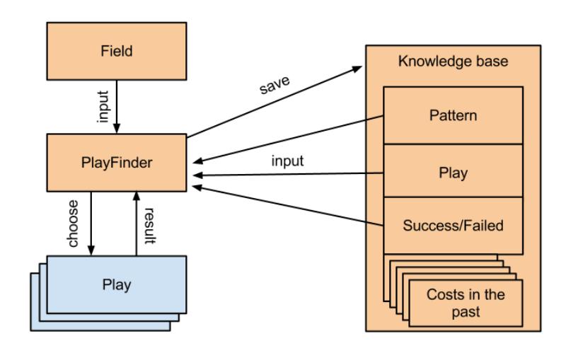
Idea overview The basic process of the play finder is depicted in figure 5. The play finder gets the current field state as input. From the knowledge base all history states can be received. One history state contains a situation of the field, a play chosen in in that situation and whether it was successful or failed. Based on this input data, probabilities will be determined for all possible combinations of plays. The set of plays with the highest score will be chosen. Furthermore, it can be regarded if the score increased in the near past, which is an indication that the actual situation is not yet reached but it will be reached in the near future. The play is then executed and reports its result back to the Play Finder. This information will be saved in the history together with the field situation.
Building up the knowledge base The knowledge base is filled during a game. Whenever a play is chosen and executed the result is saved in the knowledge base afterwards. Of course, at the beginning the knowledge base is empty, so it cannot be used for choosing a play. To have a starting point the plays are chosen randomly first. If no situation from the knowledge base matches to the current state the plays are chosen randomly. On this way, the play finder keeps on learning. If there is an unknown situation the play finder will try something and afterwards it is more intelligent because it knows the outcome of the combination from this situation and the chosen plays. The knowledge base will be persisted to a database.
Process to choose the plays The implemented play choosing algorithm is triggered for every new world frame. First, it has to be checked if new plays have to be chosen. Otherwise, the play finder does nothing. Reasons for the force of a new decision are: A play has finished, a referee command occurs, a timer has finished or when a user request occurs (for testing purposes, not possible in match mode).
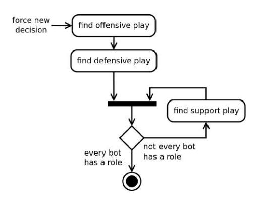
When a new decision is forced the offensive play is chosen first. This is the play which cares for the ball. If we have the ball a shooting play or another offensive play is chosen. If we are not in ball possession a play is chosen to get the ball. Next, the defensive play is chosen. This play has the task to protect the goal. It contains the role for the keeper. Last, the other bots get support plays. Figure 6 shows the described method in an overview.
The methods to find an offensive, defensive or support play are the same. The only difference is the set of the considered plays. This method does a preselection of the plays first. This means that every play is asked if it can be used in the current situation. For example, a shooting play would deny this if the enemy has the ball.
Next, the current field stored in the world frame is compared with the successful situations of the preselected plays. These situations are saved in the knowledge base. It is searched for the field with the highest similarity to the current field. This indicates that the according play worked quite well in a situation like this. Next, it is checked if the current situation has a high match in a failed situation of this play, too. This has two reasons: Perhaps exactly this situation was already chosen once. For example, if the current field was matched to 90% with a successful situation of a play it sounds like a good play to choose. However, if there is a 99% match for the same play but in this situation the play failed it does not sound so well anymore. In this case we already tried this play in nearly exactly this situation and it failed. Also it is not sufficient to rely only on the successful executions of the plays. The major part of the plays fail and there are not so many games. So there will not be a huge amount of successful executions for each play. It is necessary to get information from the failed executions, too. If there was no high match among the failed situations the play can be chosen.
Comparing field situations A field situation is a combination of bots from two teams and the ball. In order to choose plays according to a similar field situation, those must be comparable. This chapter will outline the approach that is implemented.
The overall problem when comparing those fields is, that it must be very efficient as lots of fields have to be compared. Furthermore, field situations should be as unique as possible to avoid accidental mismatches. Also it is not enough to say if two field situations are equal or not, but factor of how equal they are is required to also choose field situations that are similar, but not equal, to the current situation.
Field raster Sumatra already contains a module that is able to analyze a field raster that represents occupation of teams on the complete field. It will span a dynamic raster over the field and allows a value of 0-100 for each cell, where 0 represents full occupation of the one team and 100 full occupation of the opponent team. A value of 50 indicates equal or no occupation.
Looping over the raster and comparing differences between two field situations is quite fast and can be optimized by modifying the size of the raster, so that performance should not be a great issue with this implementation. Furthermore, the raster will already be calculated in each frame, so that the information is available without any further computation.
The field is compared cell by cell. This means, we start with the upper left cell on both field situations and calculate the difference. The differences for all cells will be summed up. The similarity factor is received by the sum divided by hundred times the number of cells, namely the maximum possible difference.
The occupation on the field is one of the most important indicators for a similar field situation, so the raster will deliver quite a good data source. However, special play patterns may not be detected. Also, there is the small chance of two rather different situations are found to be similar, as matches might be ambiguous. This is, because it will not make a great difference, on which absolute positions the bots will be located on the field as at the end, all differences will be summed up.
As this approach is a good starting point, it was chosen for final implementation with the idea of extendability of the raster in later releases.
Further considerations for the future The comparison of field situations is a fundamental part of the overall project. A lot of optimization and alternative implementations can be done. So from the beginning, we decided to build everything very modular. It is possible to place alternative implementations into the code without modifying any existing code. For now, however, there is a working and efficient implementation that will last for the first version of this learning play finder.
References
- US Digital. E4P OEM Miniature Optical Kit Encoder, 2011.
- US Digital. E8P OEM Miniature Optical Kit Encoder, 2012.
- STmicroelectronics. STM32F405xx, STM32F407xx Datasheet, 2012.
- Atmel Corporation. ATmega168P Datasheet, 2010.
- Höft & Wessel. HW86012 Product Information, 2009.
- Nordic Semiconductor. nRF24L01+ Product Specification v1.0, 2008.
- Omni Vision. OV7725 Color CMOS VGA Sensor Datasheet, 2007.
- Tigers Mannheim. TDP RoboCup 2012, 2012.
- Paul H. Vossen. Class Lecture. Learning Agents Knowledge Based Systems. Cooperative State University Mannheim, Germany. Oct. 2012.
- Paul H. Vossen. Class Lecture. Intelligent Agents Knowledge Based Systems. Cooperative State University Mannheim, Germany. Oct. 2012.
- O. Steinbrecher and P. Birkenkamp. Taktische Spielfeldanalyse im Robocup mittels Rasterung des Spielfelds, Technical report, Tigers Mannheim, 2012.