UNSAbots 2014 Team Description
Rel Guzman A., Elvis Supo C., Wilfredo Quispe I., Franco Chavez P., Eddy Amache R., Enrique Soto M., Juan Chambi M., Victor Duenas G., Percy Lovon R., Edwin Gutierrez L., Jimy C. D.
National University of St. Augustin of Arequipa, Arequipa, Peru
Abstract This paper describes the robotic system made by the team UNSAbots, for entering the Robocup 2014 competition.
1 Introduction
This is the team description paper of the Robocup Small Size Soccer Robot team "UNSAbots" for entering the Robocup 2014 competition. In this paper we present detailed description of our robots, the hardware design, as well as the software architecture in detail with focus on the software components.
This manuscript is organized as follows: Section II gives an introduction of our team and the sections. Section II describes the system overview, the mechanical structure and the electronics used for building one robot. System III describes the software architecture and the wireless communication. System IV describes the soccer strategies and the algorithms implemented for the artificial intelligence. System V describes the kinematic model implemented for the omnidirectional robot.
2 Hardware Architecture
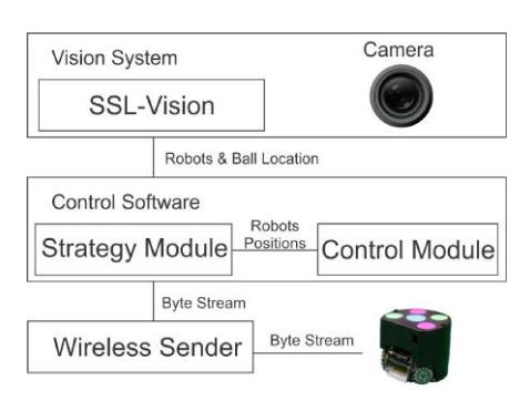
We implemented the system to receive the robots positions and the field data so we can control the robots accooring to that information, we show the system overview in Figure 1.
The hardware components of one robot are listed on Table 1.
Hardware Components
| Component | Description |
|---|---|
| Wheel | 4 vex omni wheel double roller |
| Arduino | Arduino UNO |
| Motors | 4 Motors, 12V DC, 500RPM |
| Xbee Module | Xbee module for arduino, 2.4GHz |
| Robotic Structure | Acrylic material |
2 Robocup SSL 2014
2.1 Mechanical Structure and Electronics
Our mechanical structure is based on the model made in [1]. Also the electronics are described in 1, we built a packet receiver module with arduino on each robot.
2.2 Locomotion Mechanism
A mobile robot needs locomotion mechanisms that enable it to move unbounded throughout its environment [2],
3 Software Architecture
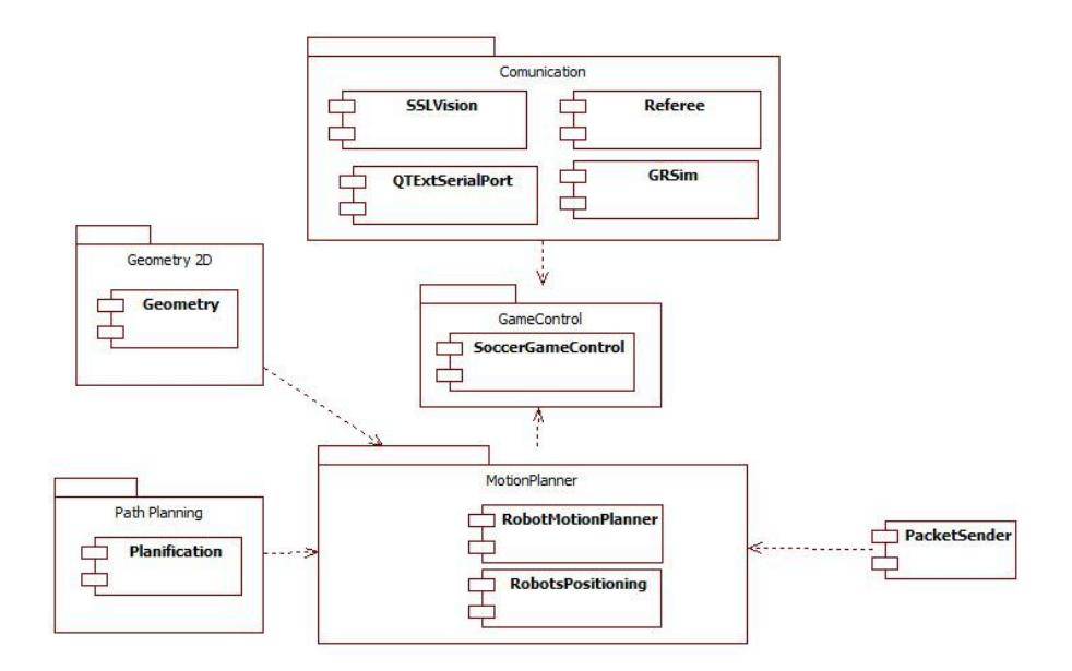
We describe our software architecture and how we we handle the information given from the real world. The overview of our software is shown as a diagram in Figure 2, and it shows the several modules organized in multi-layer.
3.1 Distributed Control
We use the Xbee module to control the robots wirelessly, and the robots can apply power to the wheels. Then the robots can work like in the simulator used.
4 Soccer Strategies
We follow the hierarchical paradigm known as Sense-Plan-Act. Players must act autonomously and also use strategies defined as plans. We define each robot as an agent, an agent is anything that can be viewed as perceiving it's environment through sensors and acting upon that environment through effectors [3].
4.1 Game State Evaluation
A right evaluation of game status plays an important role in the match. For the complexity of game situation, its really a troublesome work. We get the observation information from the ssl-vision and we save it so we can read it easily.
4.2 Path Planning and Collision Avoidance
Each robot must move around the field without hitting any other robot according to the rules. We want the robot to move from a point A to a point B and avoid colliding while doing the least expensive path [3]. We use a data structure called Quadtree to get the path in which the robot must move when moving from one point to another. The path planning algorithm is the A-star algorithm, considering the heuristic function as the distance between the initial and the target point in the path.
4.3 Goal Keeper Algorithm
The goal keeper must be sure that the ball does not enter the goal, and must be very precise in his movements. For this reason the initial position is defined a point according to the position of the ball.
- Calculate the line L defined by the points: (a) Coordinate of the ball B. (b) Coordinate of the central point in the goal G.
- Calculate the circumference with center on G and radio R.
- Calculate the point of intersection I between the point line L and the circumference.
- Calculate the angle θf between the point G and the point B
Define the target position:
$$P_f = \begin{bmatrix} I_x \ I_y \ \theta_f \end{bmatrix} \tag{1}$$
We defined a function that gets the target point and the velocity, and converts them to the velocities of each wheel.
4.4 Ball Following Algorithm
We define an algorithm like in [4], the ball following algorithm is defined according to the following steps.
- Calculate the line L defined by the points: (a) Coordinate of the ball B. (b) Coordinate of the robot R in the field.
- Calculate the angle θf from point R and the point B.
The new robot position is defined according to the distance between the ball and the robot:
$$P_f = \begin{bmatrix} I_x \ I_y \ \theta_f \end{bmatrix} \tag{2}$$
4.5 Ball Passing Algorithm
To pass the ball from one robot to another we just define the angle between the robot and the target robot and when it is on the desired angle it shoots the ball, so the other robot can keep the ball or can shoot the ball directly to the goal.
5 Kinematic Model
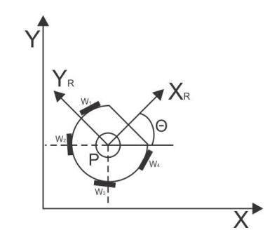
The kinematic model receives the desired end position and speed values for moving in the soccer field with precision. The process is handled directly by the software and it must send the speed of each omni-directional wheel [2]. We define two reference systems:
- X − Y : Field reference system
- Xr − Y r: Robot reference system, with reference to X, the direction of the dribbler.
As we said, the designed robot has 4 omni-directional wheels allowing us to have versatility in their movements. To perform kinematic calculations we must consider that we wish to obtain the rates at which each wheel should spin, which are represented by:
– V 0 : the first wheel speed – V 1 : the second wheel speed – V 2 : the third wheel speed – V 3 : the fourth wheel speed
And they must be obtained when we set the final position:
x0, y0 : initial position of the robot in the absolute reference system XY xf, f : final position of the robot you Jan absolute reference system XY
First, consider the address to which we want the robot to move. Also we set an angular velocity that can make the robot move while turning to the desired angle, the desired final position we have:
$$\theta_{xy} = atan(\frac{y_f - y_0}{(x_f - x_0)}) \tag{3}$$
Where:
V : Speed
θxy angle of the speed vector in the absolute reference system X − Y
W : Angular speed
Then we calculate the following:
$$V_x = |V|\cos(\theta_{xy}) \tag{4}$$
$$V_y = |V|sin(\theta_{xy}) \tag{5}$$
Where:
Vx : X-axis speed Vy : Y-axis speed
Then these parameters must shift speed values in the reference system of the robot. We must take into account a very important parameter, the initial position of the robot, represented by the angle of separation between the two reference systems, the absolute system X − Y field game and the system of internal reference Xr − Yr robot.
$$V_{yr} = |V_y|sen(\theta_{xy} - \theta_0) \tag{6}$$
$$V_{yr} = |V_y|sen(\theta_{xy} - \theta_0) \tag{7}$$
Finally, the movement of each wheel is be defined as follows:
$$V_0 = V_{yr}.cos(60) - V_{xr}.cos(30) + d.W$$ (8)
$$V_1 = -(V_{yr} + V_{xr})\cos(45) + d.W (9)$$
$$V_2 = -(V_{yr} - V_{xr})cos(45) + d.W (10)$$
$$V_3 = V_{yr}.cos(60) + V_{xr}.cos(30) + d.W$$ (11)
References
- A. Smit, "Development of a robot for RoboCup Small Size League, utilizing a distributed control architecture for a multi-robot system development platform," Ph.D. dissertation, 2011.
- R. Siegwart, I. R. Nourbakhsh, and D. Scaramuzza, Introduction to Autonomous Mobile Robots, 2011.
- S. J. Russell and P. Norvig, Artificial Intelligence: A Modern Approach, 1995.
- K. Yasui, T. Inagaki, H. Sawaguchi, Y. Nunome, H. Sasai, Y. Tsunoda, S. Matsuoka, N. Kawajiri, K. Murakami, and T. Naruse, "RoboDragons 2012 Team Description," 2012.