CMDragons 2015 Extended Team Description

Joydeep Biswas, Philip Cooksey, Steven Klee, Juan Pablo Mendoza, Richard Wang, Danny Zhu, Manuela Veloso

Carnegie Mellon University

http://www.cs.cmu.edu/~robosoccer/small/

Abstract The CMDragons team placed second out of twenty-one teams in the Small Size League of RoboCup 2014. In this paper, we present the team's recent work on the offensive and defensive tactics, low level skills, and state estimation. Among the offensive tactics, we introduce the concept of contingency options for teams of robots in the presence of uncertainty via zone-based, and support attack. We increase the robustness of the defense by creating specialized skills for handling loose balls near the defense area as well concerted multi-robot shot-blocking. We present a robot ball-manipulation skill for dribbling the ball while simultaneously turning. Finally, we describe improvements to the ball state estimation algorithms by accounting for collisions with dynamic robots.

1 Introduction

The CMDragons 2015 team from Carnegie Mellon University (Figure 1) builds upon the ongoing research from previous years (1997–2010, 2013-2014 [1]). This paper presents the technical details of our work since our Team Description Paper of 2014 [1]. The overall architecture and robot hardware have remained largely unchanged since 2010 [2, 3], and in this paper we focus on the novel contributions from this year. Our team website provides a detailed description of the robot hardware and links to technical documents from previous years.

In the following sections, we present our work related to the offense and defense tactics, ball-dribbling skills, and state estimation. Section 2 introduces the concept of contingency options in offense, and shows two applications of this concept: Zone-based Team Coordination, and a Support Attacker tactic. Section 3 presents our innovations in defense, which consist of plays and skills to defend against corner kicks, to clear stopped balls near the defense area, and to block incoming shots towards the goal. Section 4 describes a robust method for dribbling the ball while turning. We discuss improvements to ball tracker in Section 5. Section 6 summarizes the contributions and discusses future work.

2 Offensive Tactics: Contingency options

We have previously introduced robust skills for fast interception of moving balls [1], and an attacker tactic that chooses the appropriate skills to intercept and shoot the ball in the minimum possible time. However, in an adversarial domain, there are multiple possible future outcomes that depend on the exact actions taken by opponent robots. For example, if a moving ball is unlikely to be intercepted by an opponent robot, the attacker tactic could continue to use its time-optimal ball interception skill to receive the ball, while if an opponent robot is likely to intercept the ball, the attacker tactic would have to do something different, like drive up to the interception point. The attacker tactic always chooses to act on the most likely outcome, based on the current perceived world state, and the models of the opponents' capabilities. To handle the other possible outcomes, we therefore introduce contingency options for our offense: robot roles that enable offense to be robust in scenarios that are not the most likely ones. We implement this concept through Zone-based Team Coordination, and a Support Attacker tactic. The purpose of these contingency options is not to replace the primary attacker, but to complement it. While the primary attacker acts on the most likely future trajectory of the ball, Zone-based Team Coordination and Support Attacker enable offense robots to pursue other likely future trajectories of the ball.

2.1 Zone-based Team Coordination

Our team has introduced several different algorithms to coordinate offense robots. We have introduced plays as predefined team policies based on individual robot skills and tactics [5]. In this system, the plays were organized in a playbook, with weights that could be adjusted with experience [6]. In our CMDragons 2013 team, we departed from the playbook approach for planning during free kicks. Instead we introduced a coerce-and-attack planning strategy [7], an algorithm that searched for possible plans taking the opponent predicted moves into account. The core aspect of the algorithm consisted on the generation of two possible plans, one of which was revealed to induce the opponents to take positions that would open opportunities for a second viable plan. During the game, teamwork was still achieved through a playbook.

Since last year, we are focused on the research underlying the teamwork while the game is on, rather than stopped for a free kick. We have introduced a Zone-based Team Coordination in which we divide the field in several zones to be assigned to offense robots. We investigate several issues related to the definition of the zones, including (i) their dimensions and number; (ii) their degree of overlapping; and (iii) their dynamic resetting during the game, as a function of the score and time left.

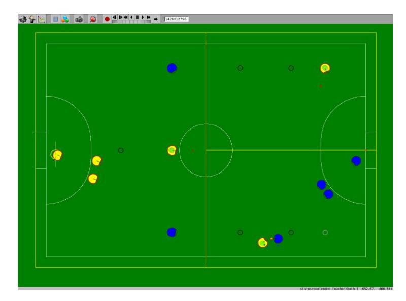
The Zone-based Team Coordination algorithm must assign robots to zones, as well as the behavior for each robot in its zone. Given a set of robots $R$ assigned to offense, we partition the field $F$ into $|R|$ zones, such that there exists a one-to-one mapping from robots to zones. Each robot $r_i \in R$ thus gets assigned to a corresponding zone $Z_i \subseteq F$ , where $\bigcup_{i=1}^{|R|} Z_i = F$ . Figure 2 shows an example of such an assignment, with three offense robots and their respective zones.

Given an assignment of zones to robots, our algorithm determines the behavior of each robot $r_i$ in its zone $Z_i$ . Let $\boldsymbol{X}_i^g$ be a set of guard positions in each zone $Z_i$ . If $r_i$ computes that the ball will enter $z_i$ , then $r_i$ moves to intercept the ball in its zone at the optimal location $\boldsymbol{x}_a(r_i)$ ; otherwise $r_i$ moves to one of the guard positions $\boldsymbol{x}_g(r_i) \in \boldsymbol{X}_i^g$ . The target location $\boldsymbol{x}_t(r_i)$ for $r_i$ is thus given by:

$$\boldsymbol{x}_t(r_i) = \begin{cases} \boldsymbol{x}_a(r_i) & \text{if } \boldsymbol{x}_a(r_i) \in Z_i \ \boldsymbol{x}_g(r_i) & \text{otherwise} \end{cases}$$

Figure 2 shows one robot intercepting the ball at its optimal location $x_a$ , and two robots placed in their assigned guard positions. We note that, when multiple robots predict the ball to be heading toward their zone, they all move to intercept it within their own zone, thus creating multiple contingency options.

We continue to investigate algorithms to set guard positions, as a function of the joint attack, the ball positioning, and the opponent positioning. Our plan is to analyze the impact of multiple alternative choices for the zone definition and robot policy assignment in extensive tests in our simulation environments.

2.2 Support Attacker

To further create contingency options in offense, we present the concept of a Support Attacker, which complements Zone-based Team Coordination: while Zone-based Team Coordination ensures good offense coverage of the field, Support Attacker provides a contingency option specifically near the ball.

The Support Attacker robot $r_{SA}$ always stays at a fixed distance $d_{SA}$ from the ball, in a direction $u_{SA}$ from which it is likely to be recover a loose ball:

$$\boldsymbol{x}t(r{\mathrm{SA}}) = \boldsymbol{x}b + d{SA}\boldsymbol{u}_{SA}$$

Our ongoing work involves investigating algorithms to determine $d_{SA}$ and $u_{SA}$ . A simple but effective assignment for $d_{SA}$ is a constant value that is large enough to not interfere with the Primary Attacker, but small enough to provide support in case the ball follows a trajectory other than the predicted most likely one. It is also possible to adapt $d_{SA}$ as a function of the current action of the Primary Attacker, or other features of the world.

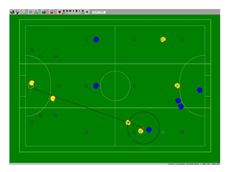
Our algorithm determines the direction $u_{SA}$ as a function of the distance from the ball at which opponents are located. If there is an opponent nearby, $u_{SA}$ is chosen to block a potential shot on our goal; if there is no opponent nearby, $u_{SA}$ is chosen to be aligned with the opponent's goal, ready to shoot. Figure 3 shows an example of a robot acting as a support attacker. We note that, even though the support attacker always tries to maintain a distance $d_{SA}$ from the ball, dynamic role assignment [5] enables a Support Attacker to become the Primary Attacker when appropriate.

3 Defense

In this year, we expanded on the threat-based defense detailed in last year's Team Description Paper [1]. We briefly summarize the defense evaluation algorithm here, to provide context for the innovations described below.

The evaluator considers the positions of the ball and the opponent robots to compute the first-level threat and several second-level threats, which are positions on the field. The first-level threat represents the most immediate means for a goal to be scored on our team. When an opponent is about to receive the ball, the first-level threat is the position of that opponent; otherwise, it is the position of the ball. The second-level threats represent possible indirect attacks on our goal; they are given by the locations of all opponents except one which is most likely to able to receive the ball first.

The available defenders are then positioned based on the locations of the threats. Primary defenders, of which there are usually two, move around the edge of the defense area, acting as the last line of defense before the goalie; secondary defenders move further out on the field, intercepting passes and shots by the opponent earlier on. The primary defenders typically defend against the first-level threat, staying between the ball and the goal; if there are two, but only one is needed to do so, the other will move elsewhere on the defense area to guard some second-level threat. The secondary defenders guard against the second-level threats; each one positions itself on a line either from a second-level threat to the goal (to block an indirect shot) or from the first-level threat to a second-level threat (to block a pass).

The computation is described in terms of tasks: each threat generates one or more tasks, each consisting of one or two positions, a priority, and other auxiliary information; the tasks are then assigned in decreasing order of priority to the available defenders. Second-level threats to block shots include two positions: one near the defense circle, in case the task is assigned to a primary defender, and one further out, for a secondary defender.

We have extended this evaluator to account for various special situations throughout the game.

3.1 Three or more primary defenders

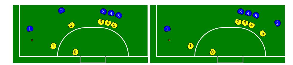
Corner kicks taken by the opponent team present a challenging problem for our defense, since opponents tend to attack with more robots than during the rest of the game, and they have an opportunity to build a play from a static ball. Assigning the appropriate defensive roles in which robots do not interfere with each other's navigation is particularly challenging when opponents quickly change formations. Figure 4 shows our solution to this, which involves assigning the role of primary defender to all our defensive robots.

This reduces the problem of positioning the defenders from a two-dimensional problem to a one-dimensional one, ensuring that the evaluator can assign positions to them in a manner which prevents collisions and interference. In this mode, the first-level threat and associated defender position or positions are computed as normal. For second-level threats, only shot-blocking tasks and only their positions near the defense are considered. All the positions are sorted by their linear position around the defense area. Now, in order to avoid collisions while allowing all robots to reach their target positions, the positions must be moved away from each other. The first-level position(s) are treated as fixed, since they represent the most important positions to block; the second-level positions are moved away from the first-level positions if necessary so that there is enough space between them for robots to reach the positions without colliding.

3.2 Clearing a stopped ball near the defense area

Since the defenders are not allowed to enter our own defense area, it is difficult for them to clear a ball which is stopped and near the area (approximately, less than one robot diameter away). One possible solution is to use their dribbler mechanisms to move the ball away from the defense area. However, this would give the opponents an opportunity to steal the ball and shoot from a close range. Instead, in this situation, the primary defenders protect the ball from the opponents while the goalie moves out from the goal to clear it.

3.3 Blocking incoming shots

When two primary defenders are positioned to block a potential shot, it is often necessary to leave a small gap between them to fully block the angle to the goal. While the goalie is positioned to block direct shots that pass between the defenders, bounces from the sides of the defenders emerge from the gap at unpredictable angles. We have solved this problem by forcing the primary defenders to quickly come together when there is an incoming shot aimed between them, reducing the likelihood that this can happen. Additionally, to prevent collisions, our algorithms evaluate which is better positioned to intercept and clear the ball. That defender then moves forward to do so, while the other stays behind.

4 Dribbling while turning

Many teams in the SSL, including CMDragons, currently dribble the ball by imparting backspin on it. This method helps the robot drive into the ball while maintaining contact with it. However, imparting backspin on the ball while turning is much more difficult than doing so without turning; in this section, we describe our ongoing effort to achieve reliable dribbling while turning quickly.

First, we describe a few intuitive approaches that fail to be robust enough while turning quickly. The first approach one could take is simply to drive around the center of the ball to turn to the desired direction. This approach works well when the ball has no spin on it, as no forces are applied on it while the robot drives around. However, when the robot has imparted backspin on the ball, the ball will roll and be lost as the robot turns around it.

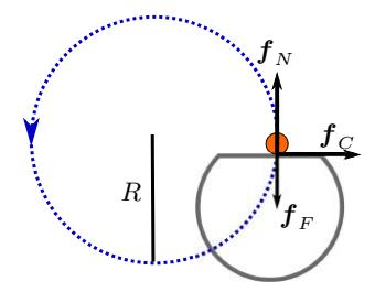
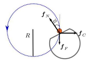
Figure 5a shows a different intuitive but ultimately insufficient approach, in which the robot drives forward with speed $s$ while gradually changing its orientation with speed $\omega$ , forming a circle of radius $R$ . These quantities are constrained by $s = \omega R$ , and which two parameters are free depend on the use of the skill. We note that the robot turning in place is a special case of this in which $R$ is the distance between the robot's center and the dribbler. As Figure 5a shows, there is no force to balance the centrifugal force experienced by the ball, and therefore the ball escapes the robot's dribbler.

Figure 5b shows our proposed approach, in which the robot turns while pushing the ball, but facing in a direction $\phi$ that provides the necessary centripetal force to maintain the ball on the dribbler of the robot: facing slightly inwards while turning provides a component of the normal force from the robot that always points towards the center of the circumference. The constraints $s = \omega R$ hold in this case as well. The necessary angle offset $\phi$ can be obtained analytically by noticing that all the forces in Figure 5b need to cancel out in the rotating reference frame. Therefore, we obtain the pair of equations:

$$|\mathbf{f}{N}|\cos\phi = |\mathbf{f}{C}|$$

$$|\mathbf{f}{N}|\sin\phi = |\mathbf{f}{F}|$$

Then, given the acceleration of gravity $g$ , the coefficient of friction of the carpet $\mu$ and the mass of the ball $m$ (which cancels out in the end), we obtain:

$$|\mathbf{f}_N|\cos\phi = m\omega^2 R$$

$$|\mathbf{f}_N|\sin\phi = \mu mg$$

Solving these equations for $\phi$ gives the result for the desired heading:

$$\phi = \tan^{-1} \left( \mu g \omega^2 R \right)$$

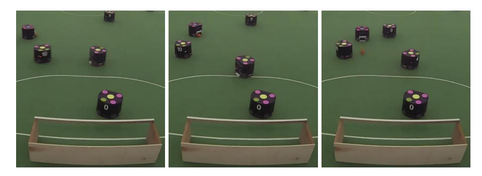
Creating a more sophisticated model, accounting for the spin of the ball, is ongoing work. However, this model showed promising results: Figure 6 shows this algorithm in action in RoboCup 2014, where it enabled multiple goals.

5 Ball tracking accounting for collisions

To track the state of the ball moving on the ground, we use an Extended Kalman Filter (EKF). While the EKF provides us with a good prediction model for the ball while it is moving freely on the ground, its predictions are less useful when the ball is about to collide with something else. This is because the EKF relies on a linearization about the estimate of the state of the ball, but collisions are highly nonlinear in nature.

Algorithm 1 Function to predict ball location accounting for collisions against robots. Input: current ball state $\boldsymbol{b}_t = (\boldsymbol{x}_t^{\boldsymbol{b}}, \boldsymbol{v}t^{\boldsymbol{b}})$ estimate and covariance $\Sigma_t^{\boldsymbol{b}}$ ; time $\Delta t$ in the future to predict ball state. Output: ball state $\boldsymbol{b}{t+\Delta t}$ estimate and covariance $\Sigma_t^{\boldsymbol{b}}$ at time $t + \Delta t$ .

1: function PredictCollisions(b_t, v_t^b, \Delta t)
 2:
               (\boldsymbol{b}_{t+\Delta t}, \Sigma_{t+\Delta t}^{\boldsymbol{b}}) \leftarrow \operatorname{PredictLinear}(\boldsymbol{b}_t, \Sigma_t^{\boldsymbol{b}})
 3:
               \boldsymbol{b}_s \leftarrow \boldsymbol{b}_t
                                                                                    ▷ record source state of current path segment
 4:
              repeat
                                                                                               \triangleright update \boldsymbol{b}_{t+\Delta t} while there are collisions
                      r_c \leftarrow \text{CollidingRobot}(\boldsymbol{b}_s, \boldsymbol{b}_{t+\Delta t})
 5:
 6:
                      if r_c \neq \emptyset then
 7:
                              (\boldsymbol{b}_s, \boldsymbol{b}_{t+\Delta t}) \leftarrow \text{Reflect}(\boldsymbol{b}_s, t + \Delta t)
 8:
                      end if
 9:
               until r_c = \emptyset
               return (\boldsymbol{b}_{t+\Delta t}, \Sigma_{t+\Delta t}^{\boldsymbol{b}})
10:
11: end function

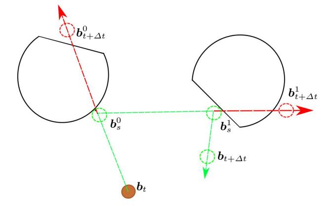
To mitigate this limitation of the EKF, we have augmented the prediction used to update it to explicitly account for the ball colliding against robots on the field. Algorithm 1 describes this process at a high level. Starting from the linear prediction of the ball trajectory (line 2), the algorithm repeatedly updates the trajectory while it finds collisions on the way (lines 4-9). For this, we find whether the trajectory intersects any robots (line 5) assuming there is at most one, and then reflect the trajectory about the point of collision (line 7). Figure 7 illustrates this process, which takes into account the geometry of the typical SSL robot (flat in the front, circular around the body) as well as typical reflection coefficients for its surfaces.

6 Conclusion

This paper presents the innovations of the CMDragons team since our last Team Description Paper [1]. Our focus has been placed on making the team more robust, by introducing the notion of contingency options on offense, expanding the abilities of defense, making our predictions of the state of the world more accurate, our skills more reliable. These innovations have allowed us to stay competitive in the RoboCup Small Size League, reaching the finals in the 2014 tournament. As we move forward, we will improve the team gameplay of our robots, introducing elements of game theory and execution monitoring.

References

1. J. Biswas, J.P. Mendoza, D. Zhu, S. Klee, and M. Veloso. CMDragons 2014 Extended Team Description Paper. In Robocup 2014.
2. S. Zickler, J. Biswas, J. Bruce, M. Licitra, and M. Veloso. CMDragons 2010 Extended Team Description Paper. In Robocup 2010.
3. J. Biswas, J.P. Mendoza, D. Zhu, P.A. Etling, S. Klee, B. Choi, M. Licitra, and M. Veloso. CMDragons 2013 Team Description Paper. In Robocup 2013.
4. Patrick Riley, Peter Stone, and Manuela Veloso. Layered disclosure: Revealing agents' internals. In ATAL-2000, July 2000.
5. B. Browning, J. Bruce, M. Bowling, and M. Veloso. STP: Skills, tactics, and plays for multi-robot control in adversarial environments. Proceedings of the IME, Part I: Journal of Systems and Control Engineering, 219(1):33–52, 2005.
6. M. Bowling, B. Browning, A. Chang, and M. Veloso. Plays as team plans for coordination and adaptation. In RoboCup 2003 Symposium, pages 686–693.
7. J. Biswas, J. P. Mendoza, D. Zhu, B. Choi, S. Klee, and M. Veloso. Opponent-driven planning and execution for pass, attack, and defense in a multi-robot soccer team. In AAMAS 2014.