TIGERS Mannheim
Andre Ryll, Nicolai Ommer, Mark Geiger, Julian Theis, Felix Bayer
Department of Information Technology, Department of Mechanical Engineering Baden-Wuerttemberg Cooperative State University, Coblitzallee 1-9, 68163 Mannheim, Germany
https://www.tigers-mannheim.de
Abstract This paper presents a brief technical overview of the main systems of TIGERS Mannheim, a Small Size League (SSL) team intending to participate in RoboCup 2015 in Hefei, China. This year the team focused on improving the artificial intelligence and the electronics of the robots. The AI core system got further improvements and several sub modules were completely redesigned. The new hardware from 2014 was reworked to fix some minor issues.
Extended Team Description for RoboCup 2015
Extended Team Description for RoboCup 2015
1 Mechanical and Electrical System
The mechanical and electrical system of our robots only experienced minor updates this year. The most important specifications are shown in table 1.
Table 1. Robot Specifications
| Robot version | 2013/2014 |
|---|---|
| Dimension | Ø178 x 148mm |
| Total weight | 2.9kg |
| Max. ball coverage | 12.3% |
| Driving motors | Maxon EC-45 flat 30W |
| Gear | 15 : 50 |
| Gear type | Internal Spur |
| Wheel diameter | 51mm |
| Encoder | US Digital E8P, 2048 PPR [1] |
| Dribbling motor | Maxon EC-16 30W with planetary gear head |
| Dribbling gear | 48 : 24 |
| Dribbling bar diameter | 12mm |
| Kicker charge topology | SEPIC |
| Chip kick distance | approx. 4m |
| Straight kick speed | max. 8m/s |
| Processors | 2x STM32F407 [2], 3x STM32F303 [3] |
| Used sensors | Encoders, Gyroscope, Accelerometer |
| Communication link | nRF24L01+ @2MBit/s, 2.400 - 2.525GHz [4] |
1.1 Reliability
Mechanical changes from the last year turned out to be very successful and reliable.
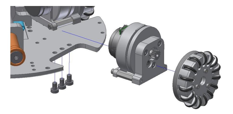
One major point was a weight reduction of the whole robot, which resulted in an increased driving performance and higher agility. The drive train was redesigned last year to form a single block, which can be exchanged as a whole including wheel, motor, encoder, and gear box. In last year's competition this provided a significant advantage in maintaining the robots. In case of a problem with any of the aforementioned parts, the drive train was fast and easily replaced (3 screws in total), allowing the robot to be back on the field within a few minutes. The exact problem could then be identified later on without impeding the game. If there is a problem with the wheel, it can be removed from the motor block individually by loosing just a single screw. Fig. 1 illustrates this process.
The electrical redesign from last year also turned out to be very reliable. Of special importance is the motor overcurrent detection. In 2013, our power electronics for the motors only used software mechanisms to present motor overcurrent situations, i.e. measure the current with an ADC and switch off the power stage in overcurrent situations via the microcontroller. This solution is prone to software problems and can also be too slow for short-circuit situations, resulting in severe motor and board damage in 2013. The 2014 electronic design uses a shunt-based overcurrent detection mechanism from the power stages' gate drivers (IRS23364 [5]). This is a purely analog solution without any microcontroller involvement. A low-pass filter allows short overcurrent situations for e.g. starting the motor, but prevents them for extended periods of time. The limit is currently set to 4A.
This safety mechanism, among others, made the electronics very reliable and most boards from last year's competition are still in use. A detailed overview of the electrical system and its safety features (also for the high-voltage kicker circuit) can be found in our 2014 TDP [6].
1.2 Planned Improvements
This year's electrical update will focus on sensor noise reduction, battery protection, and component size and quantity reduction (lower total price). Especially, the motor current measurements were not used up to now, simply because they were too noisy to be a reliable source of information. This problem will be mitigated by replacing the switching regulator for the main 3.3V supply line by a linear one. Although it has a higher current consumption, its noise absorbing properties are most important. The supply voltage from the battery will be converted to 5V with a switching regulator, and from there to 3.3V with the LT3080 linear regulator. Additionally, EMI filters, ferrit beads, and LC low-pass filters are now used at critical components to block noise from other components and from the environment.
Another important point is the protection of the battery, especially against deep-discharge situations. Although we observe the battery voltage and switch off the motors at a certain threshold, the robot remains on. The microcontrollers are still consuming enough power to deeply discharge the battery. A situation that should be desperately avoided with Lithium-Polymer batteries. To mitigate this problem we are now using the LTC4231 Micropower Hot-Swap Controller [7] to monitor battery voltage and current consumption of the whole robot. In case of a total current consumption of more than 33A or a battery voltage below 9V, the power supply is deactivated and the robot enters a shutdown state. In this state, the total current consumption is below 1µA. In conjunction with the LTC2955 On/Off Controller [8], this combination also allows the microcontroller to power off the whole robot. This command can also be issued remotely from our central software to switch off all robots at once. The batteries may then remain connected in the robots. This significantly eases the handling process of multiple robots.
Apart from electrical changes, we are also investigating options to dampen our electronic boards to make them more resistant to mechanical stress (e.g. robot and ball impacts). The idea is to mount the electronics on silicone gel pads. On the one hand, this will absorb heavy impacts, which are usually directly transferred to all components due to the stiff structure of the robot. On the other hand, this will also reduce vibrations from the wheels (which are not perfectly round due to their omniwheel structure). These vibrations have a direct effect on the quality of the gyroscope and accelerometer data and therefore the control performance of the robot.
2 Software
We use the same software framework that we created for our first RoboCup 2011, but it has grown significantly since 2011. The software allows developers to easily visualize strategies on a 2D field with few lines of code. A log recorder is able to capture all AI data, store it on disk and play it back, even if data structure has changed in code. We use Oracle Berkeley DB for Java, which supports automatic persistence of objects without defining any data structures for persistence and a high performance architecture[9]. This enables us to watch AI decisions step by step and to visualize the interesting parts while hiding everything else. In combination with the ability to let our AI play against itself and a simple automatic referee system that sends basic referee commands and replaces the ball in the simulator, we are able to test the AI extensively.
2.1 AI concept
Last year we introduced a new AI concept. It is described in our TDP from 2014[6] in more detail. The most important change was the removal of the idea of hard coded plays with the aim of faster reaction time towards quickly changing situations. We wanted to focus on single roles instead. An offense role deals with the ball and decides on demand what to do, the support role finds good positions on the field to support the offense role, the defender role blocks the defense area or any opponents and the keeper role defends the goal. We were very satisfied with this concept and it probably helped us reaching the top 8 in 2014, so we will stick to it this year. We will, however, rework the individual components for 2015. The changes are summarized in upcoming sections.
In addition to the roles, a major component in the new AI is the role assigner that switches roles among robots. The implementation from last year turned out to be too complicated and too hard to maintain, so we simplified this module now and focused on stability.
2.2 Role Assigner
The task of a role assigner is to assign roles to individual robots. It has to decide on how many roles to use for each type, depending on the current situation and the number of available robots. The implementation of last year used several algorithms, that were independent from the other AI modules, to determine the best assignment. It turned out that without any communication between roles and assigner, there were significant drawbacks. Algorithms may result in different decisions and might even misbehave, because they are not tested and maintained as good as the main implementation.
Thus we built a new role assigner that focuses on stable assignment and provides an interface to AI so that it can use hints from main logic and try to satisfy assignments to certain constraints. The whole role assigner is roughly summarized in algorithm 1. The AI modules can define the number of roles they need at least (minRoles), how many they would like to have (desiredRoles) and how many they could deal with at most (maxRoles). Additionally, they can suggest some desired bots that they would like to get assigned. The role assigner tries to satisfy those hints. If there are impossible combinations, plays with the highest priority are preferred. The advantage of this approach is that there is no specific logic within the role assigner module. It does not make any assumption upon the behavior of the plays. This makes it easier to understand the behavior of the role assignment for people who work on their own AI modules.
The changes turned out to be very helpful for AI developers because of before mentioned reasons.
Algorithm 1 New role assigner for 2015, focused on simplicity and stability.
Require: plays ∈ {OF F ENSE, SUP P ORT, DEF ENSE, KEEP ER}
Require: minRoles, maxRoles, desiredRoles, desiredBots
1: sort plays by priority, highest first
2: remove desiredBots with lower priority
3: for all plays as play do
4: play.numRoles += minRoles(play)
5: end for
6: for all plays as play do
7: play.numRoles += min(desiredRoles(play), rolesLeft)
8: end for
9: for all playsas play do
10: fill up roles until maxRoles(play) reached or no roles left
11: end for
12: for all plays as play do
13: add or remove roles from play to fit new play.numRoles
14: end for
15: for all plays do
16: Assign desiredBots if not already assigned
17: Keep assignments from last frame if possible
18: Assign unassigned roles to available bots
19: end for
2.3 Offensive
Our offensive strategy has been completely redesigned. Last years offensive strategy was pretty simple. We had only one active offense role interacting with the ball at a time. We thought that our AI is fast enough to handle very quick switching between offense roles, but having only one offense role made passing quite complicated. So we implemented a new offensive strategy which can handle more than one robot. Most of the time there will still be only one active role. This role is always ball oriented and tries to obtain ball control. As soon as the robot is close enough to the ball, it will decide what further actions should be taken. Possible offensive actions are:
- A direct shot on the goal
- A pass (straight or chip) to another TIGERS bot
- A chip kick into the enemy's half to disarm a dangerous situation
- A pull back skill to conquer the ball from enemy robots
- A special moving kick with heavy dribbler usage
The decision-making depends on several indicators:
- The width of the free direct shoot corridor
- The distance to the enemy's goal
- The distance of enemy robots to our offense role
- The chance of success for a pass to a potential supporting bot
- The direct shot scoring chance of potential pass receiving robots
- The location of the ball ( e.g. inside the penalty area )
In case of a pass, the AI will add a second offensive robot to receive the pass. One big improvement is that now this robot is assigned before the pass is on its way. This means the robot has much more time to align itself. The pass receiving robot can even move to another free location to outplay enemy robots. Thus the shooting robot can pass to the target position of the receiver. We have implemented a new ball analyzer module (see section 2.6) to predict the movement of the ball, this helps the offensive role to intersect the balls movement path and even to shoot or catch fast moving balls.
2.4 Support
Apart from the TIGERS Mannheim's soccer robots on defense and offense positions, the remaining bots act in a supporting role. Their job is mainly to be available as passing targets and redirectors in offensive situations, but could also be used to disrupt the opponents play to enhance defensive effectivity.
The most challenging problem in achieving this is to successfully break free from opponent bots, which may be following a man-to-man marker strategy while at the same time getting to a good position in order to redirect a pass or even better - score an immediate goal. Advanced tactics could include things like moving supporting bots to positions such that opponent defenders get engaged in false attacks and a path to the goal is cleared for a real offensive play. The other way round, support bots can block opponent offensive plays far from our own penalty area.
Previous attempts (as could be seen during the RoboCup 2014 in Brazil) used the processing power of a graphics card to compute a score reaching from zero to one for every single point of a grid laid over the whole field. While a value of zero represented a perfect location and one a "forbidden" area, a hill climbing algorithm was used to estimate an optimal target nearby of the bot in question. Due to the powerful function used to calculate the single scores being able to be adjusted to various different parameters such as weighting and tolerance of distance to goal, ball and opponent robots or visibility to goal or possible further pass receivers, this method used to show a quite flexible behavior. It also delivered promising results in simulations and on our laboratory test field.
However, the approach proved to have some major drawbacks. Most of all, in the highly dynamic situation of a RoboCup game the calculated scores for every point can change very fast, and so do the local optima. This would result in a lot of often unnecessary and unpredictable movement of our support bots. Additionally, it turned out to be hard to adjust the algorithm's behavior the way we wished, since the huge amount of parameters would always develop various side effects in different combinations.
To achieve a more effective and controllable behavior, we chose to abandon our old calculators and completely redesign the support role. It does now also resemble a real assisting footballer's strategy much closer: Each support role checks its own environment for several possible good positions to receive and redirect passes. If such exist, it does not move there since an opponent defender could easily follow and intercept incoming passes or the enemy goal keeper could prepare to block (indirect) goal shots. Instead, the support roles offer their potential pass-receiving positions to the offense role. The offense role then chooses the estimated very best passing target from these positions. Only the moment it decides to really pass the ball on, the support bot becomes a second offensive player and moves to the passing target to receive the passed ball.
Every bot's potential pass receive points are simply calculated and evaluated regarding distance and angle to ball, goal and the bot's kicker location itself. If there is no point found for a support bot, it chooses a different position, checks if points are available there and eventually moves there.
The strategy used to find new positions can be configured by dependency injection. At the moment a fast solution is based on random generated locations, but more elaborated algorithms are in development. For example, a machine learning algorithm could be applied to prefer support bot constellations from which the opponent team proved to suffer defensive weaknesses.
2.5 Defense
The aim of the defensive bot is to prevent the enemy bots from scoring any goals. More extensive aims are to prevent the enemy from passing the ball and prevent the build-up of the enemy's game.
In the past years two of our defensive bots were covering the line between the enemy bot which possessed the ball and our goal. Every other defensive bot was covering an enemy bot that was located at a good position to score a goal in case it received the ball. The covering bots were all located at the scope of our penalty area. An algorithm determined pairing between our bots and the enemy bots. It sorted our bots and the enemy bots respectively from the top to the bottom of the field. Our topmost bot was commanded to cover the topmost enemy bot and so on.
Through this strategy we built a dense wall around our penalty area. The enemy was to play a sophisticated offensive passing strategy to get past our defense line.
The disadvantages of this strategy were that the enemy got a free field to build up its plays and look for holes in our defense. Furthermore, our defenders were not moving the shortest cumulated way, so the enemy got some time to score a goal before our defense line was built up.
The goals for our new defensive strategy are:
- to position our defensive bots faster by shortening the way that every defender moves
- to play a more "offensive" defense strategy by positioning our bots in more offensive positions
- to interrupt the enemy's game by blocking possible paths of the enemy bots and pass paths
- to implement a more modular defense in order to switch between different defensive strategies and adapt to the enemy's plays
The build-up of the defense is organized in a cycle consisting of three steps:
- generating some information about every enemy bot and the possible interactions between the enemy bots
- creating a list of the most dangerous enemy bots
- calculating a mapping between our defensive bots and the best possible defensive positions
In the first step the goal is to create as much useful information about the enemy's game as possible. This information is used by the calculators in the other steps. For every enemy bot its vector to our goal is stored. In this vector the nearest possible point to our goal, restricted by the penalty area, and the nearest point to the enemy bot, restricted by the bot's radius, are stored. In addition to that, the intersections between these vectors and the vectors between the enemy's bots (possible passing paths) are saved.
The second step is about creating a list of the enemy bots posing the greatest threat to our goal. Several calculators can be used to calculate the threat of every enemy bot. We created an interface to a calculator class that every calculator in this step has to implement. Every implementation of the interface uses different indicators, or a combination thereof, to determine the threat posed by every enemy bot. Possible indicators are:
- the distance between the enemy bot and our goal
- the angle of the enemy bot to our goal
- the distance between the enemy bot and the ball, or even possession of the ball by the enemy bot. The possession is determined by a very short distance between the bot and the slowly-moving ball
- the enemy bot's possibilities to move
- the enemy bot's possibilities to receive a pass
The enemy bots are sorted by the threat posed by them and stored in a sorted list. The calculators can be switched dynamically to use the calculator most suitable to the enemy's tactics. In the third and last step, for each of our defensive bots the best defensive position, determined by a calculator, is assigned.
The calculation is performed by one of several calculator classes inheriting from a common base class. The calculator class has to implement a single method that gets the information calculated in the first two steps and a list of defender bots. It returns a mapping of the defender bots to their relative defense position. The positions can be calculated in many different ways, regarded information being:
- the shortest cumulated distance
- the vector from an enemy bot to our goal
- the vectors between the enemy bots
- the ability of an enemy bot to move
- the area covered by our defenders
- the possibility to shorten a pass or shoot angle of an enemy bot
- the tactics of the enemy team
Using this information every calculator class uses different approaches to achieve the best defense. The calculators can be switched dynamically. As an example, a rather sophisticated calculator class is described. In the beginning, the bot closest to the vector from the ball-nearest enemy bot to our goal gets paired with the nearest point on this vector. Using a Steinhaus–Johnson–Trotter algorithm every possible combination of our defenders and their respective nearest point on the vector of the most dangerous enemy bot is calculated. The mapping with the shortest cumulated distance is chosen. This information is considered important for interrupting the enemy bot's shot vector. If this is the case, the position on this vector is optimized. The calculator tries to find a point on the vectors or every bot to interrupt as many passing opportunities as possible. The defender covering the enemy bot possessing the ball gets assigned the point nearest to the enemy bot to try to conquer the ball. The general construction of the defense allows to introduce new calculators and therefore a new behavior of the defense easily. The hope is to construct these new calculators in short development cycles and to verify them in test games and the simulator. The calculators can be switched by the software in-game or during timeouts to adapt to an enemy's tactics.
2.6 Analyzing the ball movement
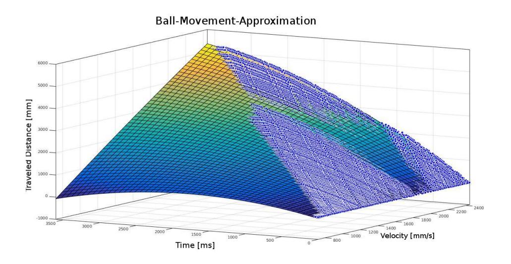
To efficiently obtain ball control or to kick a moving ball it is mandatory to know where the ball will be after a specific period of time. We created a new module to analyze the ball movement more accurately than before. Now we are able to calculate the future ball position or velocity within a very small tolerance. We can even determine the exact position where the ball will come to a standstill. The algorithm will also work in different environments (carpets). With a small training phase the algorithm can adapt to the new situation. Our AI tracks and records the position, the velocity and the time stamp for each frame. When enough data has been collected, our AI calls an external Matlab script which does some further processing. First of all, the script will soften the recorded data by eliminating spikes and inaccurate data points. Then the script generates a new set of data points, reaching from the current (initial) velocity to the last recorded velocity, for each recorded frame. This creates a triangle-shaped cloud of data points (blue dots in Figure 2).
The script will then do some curve fitting, using the Matlab curve fitting tool, to approximate a function which can estimate the distance traveled by the ball after a given time y with a given initial velocity x.
Figure 2 shows a polynomial regression function of a big set of collected movement data. The blue dots represent the collected data and the blue/yellow surface the approximated function. Formula 1 shows the approximation function, where pij are the automatically generated parameters of the fitting surface. For now the validity of the parameters pij have to be checked manually.
The calculated parameters for the fitting surface will be returned to our AI module automatically. With formula 1 we can determine the future ball position. Formula 2 shows the derivative of Formula 1.
$$\text{distance} = p_{00} + p_{10} \cdot x + p_{01} \cdot y + p_{20} \cdot x^2 + p_{11} \cdot x \cdot y + p_{02} \cdot y^2$$
$$y = (((vel_{end} - (2 * p20 * x) - p01) + (p11 * x)) - p10)/(p11 + (2 * p02))$$
With formula 2 we can calculate the time in which the ball will reach a given velocity (velend). By rearranging those formulars lots of interesting methods can be created. We have implemented quiet a few methods using this approximation Formulars. For example: getPosByTime(), getPosByVel(), getTimeByPos(), getVelByPos(), getVelByTime(). With this information we can build more precise kicking and defending skills.
3 Publication
Our team publishes all their resources, including software, electronics and mechanical drawings, after each RoboCup. They can be found on our website. The website also contains several publications about the RoboCup, though some are only available in German.
References
- US Digital. E8P OEM Miniature Optical Kit Encoder, 2012. http://www.usdigital.com/products/e8p.
- STmicroelectronics. STM32F405xx, STM32F407xx Datasheet, 2012. http://www.st.com/web/catalog/mmc/FM141/SC1169/SS1577/LN1035/PF252144.
- STmicroelectronics. STM32F302xx, STM32F303xx Datasheet, June 2013. http://www.st.com/web/catalog/mmc/FM141/SC1169/SS1576/LN1531/PF253449.
- Nordic Semiconductor. nRF24L01+ Product Specification v1.0, 2008. http://www.nordicsemi.com/eng/Products/2.4GHz-RF/nRF24L01P.
- International Rectifier. IRS2336(D), IRS23354(D) High Voltage 3 Phase Gate Driver IC, April 2011. http://www.irf.com/product-info/datasheets/data/irs2336.pdf.
- A. Ryll, N. Ommer, M. Geiger, M. Jauer, and J. Theis. TIGERS Mannheim - Team Description for RoboCup 2014, 2014.
- Linear Technology. LTC4231 Micropower Hot Swap Controller Datasheet, 2014. www.linear.com/LTC4231.
- Linear Technology. LTC2955 Pushbutton On/Off Controller with Automatic Turn-On Datasheet, 2012. www.linear.com/LTC2955.
- Oracle Corporation. Berkeley DB Java Edition Architecture, 2006.