CMDragons 2016 Extended Team Description Paper
Juan Pablo Mendoza, Joydeep Biswas, Danny Zhu, Richard Wang, Philip Cooksey, Steven Klee, Manuela Veloso
Carnegie Mellon University
http://www.cs.cmu.edu/~robosoccer/small/
Abstract The CMDragons Small Size League (SSL) team won all of its 6 games at RoboCup 2015, scoring a total of 48 goals and conceding 0. This paper presents the core coordination algorithms in offense and defense that enabled such successful performance. We first describe the coordinated plays layer that distributes the team's robots into offensive and defensive subteams. We then describe the offense and defense coordination algorithms to control these subteams. Effective coordination enables our robots to attain a remarkable level of team-oriented gameplay, persistent offense, and reliability during regular gameplay, shifting our strategy away from stopped ball plays. We support these statements and the effectiveness of our algorithms with statistics from our performance at RoboCup 2015.
1 Introduction
The CMDragons 2015 team from Carnegie Mellon University builds upon extensive research from previous years (1997–2010 [1,2,3], 2013–2014 [4]), in areas including computer vision [5], path [6] and dribbling [7] planning, execution monitoring [8] and team architecture [9]. This legacy enables our 2015 team to focus on the problem of coordinated decision-making for a team in a highly dynamic adversarial domain. Furthermore, while previous years have seen a focus on stopped-ball plays [10], this year our team focuses its research efforts on regular gameplay team planning. As a result, our offensive strategy relies heavily on teamwork, with 245 pass attempts and 194 completions over the tournament.
To achieve such coordination, our algorithms are divided into various layers:
- The coordinated plays layer [9] decides how many robots are assigned to a defense subteam and to an offense subteam, based on functions of the state of the game.
- Each of these two subteams creates coordinated plans to maximize the team's probability of scoring and not being scored, respectively.
- Each robot individually selects actions that are consistent with the coordinated plan and maximize the probability of success.
- The robots execute these actions through various new reusable skills [10].
This paper focuses on the team coordination layers of items 1 and 2: Section 2 discusses the coordinated plays layer, while Sections 3 and 4 discuss the coordinated plans of offense and defense, respectively. In Section 5, we analyze the performance of these algorithms at RoboCup 2015, through various statistics extracted from the tournament. These statistics show how our team (a) maintained persistently offensive gameplay throughout the tournament, (b) successfully executed a team-oriented strategy, and (c) significantly increased its focus on regular gameplay, as opposed to stopped ball gameplay.
2 Coordinated Plays Layer
At the top coordination level, our algorithms divide the team of robots into two subteams: the defense robots, whose goal is to minimize the probability of the opponents scoring a goal on our team, and the offense robots, whose goal is to maximize the probability of scoring on the opponent team. The number of robots assigned to each of these subteams reflects the desired level of aggressiveness for the current situation.
We specify this subteam division through plays [11], each of which is defined by (a) the n roles that the n robots should fill, and (b) the applicability conditions for choosing that play. The CMDragons 2015, playing with n robots, used plays with either 1, n-3, or n-2 offense robots; the team switched among these plays according to the desired level of aggressiveness, as defined by the play applicability conditions. These applicability conditions are based on three functions of the state of the game: ball possession ballP, field region fieldR in which the ball is located, and the opponent's level of aggressiveness oppA.
Ball Possession: Variable ballP can take one of four values: ourB, theirB, contendedB, or looseB. We estimate the possession state ballP_t at time t using the length of time $t_{\text{near}}^{\text{us}}$ and $t_{\text{near}}^{\text{them}}$ that the ball has been closer than $d_{\text{near}}$ to us and the opponent, respectively, and the time $t_{\text{far}}^{\text{us}}$, and $t_{\text{far}}^{\text{them}}$ that the ball has been farther than $d_{\text{far}}$ from us and the opponent, respectively:
$$\mathbf{ballP}{t} = \begin{cases} \text{ourB} & \text{if } (t{\text{near}}^{\text{us}} > t_{\text{near}}^{\text{thresh}}) \wedge (t_{\text{near}}^{\text{them}} < t_{\text{near}}^{\text{thresh}}) \ \text{theirB} & \text{if } (t_{\text{near}}^{\text{us}} < t_{\text{near}}^{\text{thresh}}) \wedge (t_{\text{near}}^{\text{them}} > t_{\text{near}}^{\text{thresh}}) \ \text{contendedB} & \text{if } (t_{\text{near}}^{\text{us}} > t_{\text{near}}^{\text{thresh}}) \wedge (t_{\text{near}}^{\text{them}} > t_{\text{near}}^{\text{thresh}}) \ \text{looseB} & \text{if } (t_{\text{far}}^{\text{us}} > t_{\text{far}}^{\text{thresh}}) \wedge (t_{\text{far}}^{\text{them}} < t_{\text{far}}^{\text{thresh}}) \ \ \mathbf{ballP}_{t-1} & \text{otherwise} \end{cases}$$
where $t_{\text{near}}^{\text{thresh}}$ and $t_{\text{far}}^{\text{thresh}}$ are time thresholds.
Field Region: Variable fieldR attains one of two values: ourH and theirH, according to the half of the field in which the ball is located.
Opponent Aggressiveness: If the opponent has 0 robots in our half of the field, then $\mathbf{oppA} = \mathrm{def}$ ; otherwise, $\mathbf{oppA} = \mathrm{off}$ .
Table 1 illustrates how the CMDragons divide the team into offense and defense based on these functions of the state of the world. When the ball is in our half of the field, and we do not have possession of the ball, we enter a very defensive play. When the ball is in the opponent's half of the field or the opponent has no robots in our half, and the opponent does not have possession of the ball, we enter a very aggressive play with n-2 offense robots. In all other circumstances, our team plays with 3 defense robots and n-3 offense robots.
Table 1: Play choice based on the state of the game. Usually, the team is of size n = 6, but n < 6 is possible due to cautionable offenses or mechanical problems.
| Game state | Offense Size | Defense Size |
|---|---|---|
| $\mathbf{fieldR} = \mathbf{ourH} \wedge \mathbf{ballP} \neq \mathbf{ourB}$ | 1 | n-1 |
| $(\mathbf{fieldR} = \mathbf{theirH} \lor \mathbf{oppA} = \mathbf{def}) \land \mathbf{ballP} \neq \mathbf{theirB}$ | n-2 | 2 |
| All others | n-3 | 3 |
3 Offense Coordination: Zone-based Selective Reactivity
The CMDragon's multi-robot coordination algorithm, which is in large part responsible for the team's success in 2015, is the product of years of research and change. Here, we describe how our 2015 offense algorithm emerged as a combination of our 2013 and 2014 algorithms, achieving a balance between being reactive to the opponent's actions and assertive in carrying out its own plans.
3.1 CMDragons 2013: Reactive Offense
Our 2013 offense emphasizes reactivity toward the opponents. Given the set R of offense robots, 1 Primary Attacker (PA) robot handles the ball using one of two actions: shoot it on the goal or pass it to a teammate; the remaining |R|-1 Support Attacker (SA) robots navigate to their estimated optimal location to receive a pass from the PA. All |R| robots are thus highly reactive to the opponents: the PA's decision depends on whether the opponents have left a good shot on the goal open, and on whether the passes to its teammates are likely to succeed; the SAs' receiving location x* depends on how likely the opponents are to intercept a pass to x* given their current configuration, and how likely a goal is to be scored from x*, given the opponents' configuration. Details on these computations can be found in previous work [10].
Such reactivity is a desirable quality, since it enables our robots to choose effective actions in different scenarios. Pure reactivity, however, prevents our robots from generating and carrying out their own plans. Furthermore, since our SAs continuously move in reaction to the opponent to the estimated optimal passing location, and most defending opponents also continuously move in reaction to our robots to prevent them from reaching an effective passing location, the state of the world is constantly and rapidly changing, which complicates the problem of accurately passing and coordinating. Thus, we decided to explore less reactive algorithms that would give our offense more control over the evolution of the state of the world.
3.2 CMDragons 2014: Fixed Zones and Guard Locations
Our 2014 offense emphasizes our team's assertiveness in controlling the evolution of the game in a more predictable way. To this end, we introduced a Zone-based Team Coordination algorithm [12], which we briefly describe here.
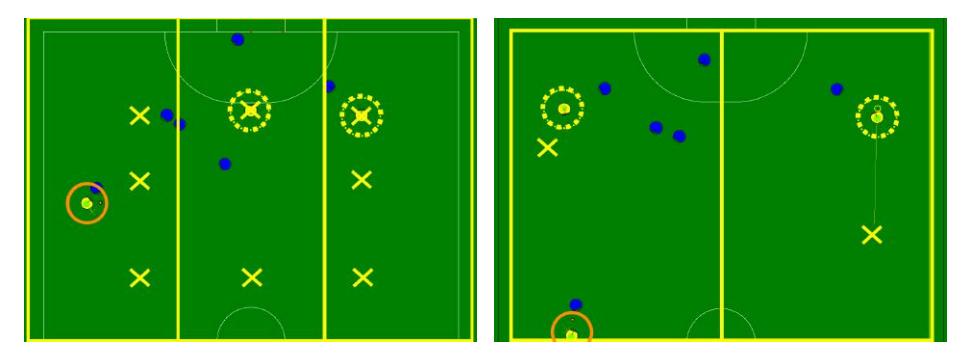
The algorithm partitions the field F into |R| zones, such that there exists a one-to-one mapping from robots to zones. Each robot $r_i \in R$ thus gets assigned to a corresponding zone $Z_i \subseteq F$, where $\bigcup_{i=1}^{|R|} Z_i = F$. Figure 2a shows an example of such an assignment, with three offense robots and their respective zones.
Given an assignment of zones to robots, the algorithm determines the behavior of each robot $r_i$ in its zone $Z_i$. Let $\boldsymbol{X}_i^g$ be a set of guard positions in each zone $Z_i$. If $r_i$ computes that the ball will enter $z_i$, then $r_i$ moves to intercept the ball in its zone at the optimal location $\boldsymbol{x}_a(r_i)$; otherwise $r_i$ moves to one of the guard positions $\boldsymbol{x}_g(r_i) \in \boldsymbol{X}_i^g$. The target location $\boldsymbol{x}_t(r_i)$ for $r_i$ is thus given by:
$$\boldsymbol{x}_t(r_i) = \begin{cases} \boldsymbol{x}_a(r_i) & \text{if } \boldsymbol{x}_a(r_i) \in Z_i \ \boldsymbol{x}_g(r_i) & \text{otherwise} \end{cases}$$
Figure 2a shows one robot intercepting the ball at its optimal location xa, and two robots placed in their assigned guard positions. These guard positions were determined empirically prior to the games, and were independent of the state of the opponent. Thus, the offense is indifferent to the opponent in its decisions, save for the ball-handling robot, which still decides whether to shoot or pass based on the full state of the world.
This indifference to the state of the opponents gives our 2014 offense more control over the state of the game by enabling pre-defined plans to be carried out, and settling the game into a more slowly-changing pace. However, the lack of reactivity to the opponent has drawbacks, since robots make no effort to improve the probability of scoring by moving to better locations on the field.
3.3 CMDragons 2015: Zones and Reactive Positioning
In 2015, we created an algorithm that combines the strengths of our 2013 offense and our 2014 offense, and awarded the PA more freedom on the field and action options. This coordination algorithm is also zone-based, but the number of zones, their coverage of the field F, and the behavior of each robot given these zones is different. Given R, the algorithm creates |R| − 1 zones, which affect the robots' behaviors as described below.
Primary Attacker (PA): One robot is assigned to the role of PA, and is the only robot that handles the ball to shoot on the opponents' goal, pass to a teammate, or keep the ball away from opponents while creating passing or shooting options. The PA is not bound to a zone.
Support Attackers (SAs): Each of the remaining |R|-1 robots $r_i$ is assigned the role of SA within a zone $Z_i \subseteq F$. Similarly to the 2013 algorithm, each $r_i$ estimates the optimal location $\boldsymbol{x}^(r_i)$ to receive a pass; however, the search is constrained to locations in $Z_i$, such that $\boldsymbol{x}^(r_i) \in Z_i$. Similarly to the 2014 algorithm, we define a set of guard positions $\boldsymbol{X}_i^g \subset Z_i$. Then, the target location of robot $r_i$ is given by:
$$\boldsymbol{x}_t(r_i) = \begin{cases} \boldsymbol{x}^*(r_i) & \text{if PA is ready to pass to } r_i \ \boldsymbol{x}_g(r_i) & \text{otherwise} \end{cases}$$
The evaluation deciding whether the PA is ready to pass to $r_i$ is made using a pass-ahead coordination algorithm [10] that prevents $r_i$ from moving to $\boldsymbol{x}^*$ too early or too late for the pass.
Using this algorithm, our team is able to create and carry out plans independently of the opponent by choosing the zones $Z_i$ and the guard positions $X_i^g$; this enabled our 2015 team to create sequential plans in which the sets of zones assigned to the SAs evolved to move the ball towards the opponents' goal [13]. At the same time, the offense maintains high reactivity to the opponents, since the SAs always search for the best receiving location $x^$ within their zone $Z_i$. Importantly, however, the SAs only start moving toward $x^$ at the last safe moment, according to the pass-ahead coordination; thus, our SAs, and thus usually the opponents marking them, are usually more static and predictable.
Figure 2b shows an example of our 2015 algorithm: The SA on the left half waits in its guard location, since the pass-ahead coordination has computed that it should not start moving yet. On the other hand, the SA on the right half has computed it must start moving to its receive location, and thus has started navigating away from its guard location (yellow circle) toward its receive location (red and black concentric circles).
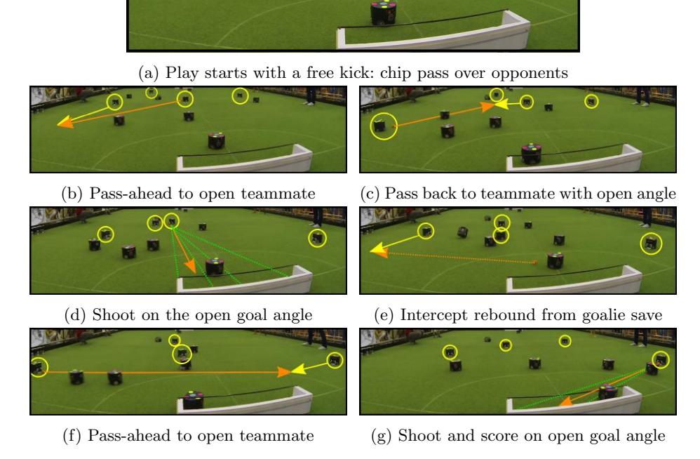
Figure 3 shows an example of our offense coordination in RoboCup 2015, illustrating the results described in Section 5: our coordinated offense exhibits (a) successful teamwork through multiple passes, (b) offensive persistence by maintaining possession on the opponent's half and repeatedly shooting on open angles on the goal, and (c) regular gameplay effectiveness by keeping the ball in play over multiple passes, shots, and a rebound off the opponent.
3.4 Other Offense Contributions
In addition to the offense coordination algorithm presented, CMDragons 2015 includes several other features that greatly supported the success of our team: (a) an extremely dedicated care of our 10-year old robot hardware; (b) scripted plays with dynamic zones tuned by extensive simulation games ahead of the tournament and enabled by our novel autoref algorithm [14]; (c) carefully polished action execution; (d) online adaptation of free kick plays according to observed performance metrics [15]; and (e) novel individual robot skills to enable the dribbling the ball, and intercepting any free ball, independently of its origin.
4 Defensive Coordination: Threat-based Evaluation
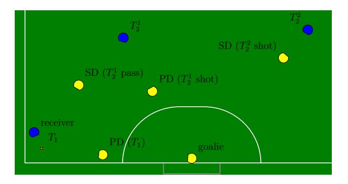
Our defense relies on a threat-based evaluator [10], which computes the first-level threat T^1 and several second-level threats T_i^2 on our goal: T^1 is the location from which the opponent can most immediately shoot on our goal — i.e., the location of the ball, if it is stationary, or the location of the robot that will receive the ball, if the ball is moving. Threats T_i^2 are locations of opponent robots that might receive a pass from the T^1 robot, and then shoot on our goal.
The available defenders are positioned based on the locations of the threats. Primary defenders (PDs), of which there are usually one or two, move near the defense area, acting as the line of defense before the goalie; secondary defenders (SDs) move further out, intercepting passes and shots by the opponent earlier on. The PDs typically defend against the T1, blocking open goal angles between the ball and the goal; if there are two PDs, but only one is needed to block a potential shot, the other moves elsewhere on the defense area to guard a T2. (This situation arises when the ball is close to one of the near corners of the field.) The SDs guard against the various $T_2$s; each one positions itself on a line either from a $T_2$ to the goal (to block a shot) or from the $T_1$ to a $T_2$ (to block a pass). Depending on the number of available defenders, our algorithm first selects up to two robots to the role of PD, and then assigns the remaining defense robots to the role of SD. Figure 4 shows the $T_1$ and $T_2^i$, and the corresponding PD and SD assignments for a particular state of the world.
The aim of the goalie and the defenders guarding the $T_1$ is to entirely block the open angle from the threat to the goal; if this is not possible, they position approximately so that as much of it as possible is blocked.
4.1 Defense Behavior Illustration: 5 Defense Robots
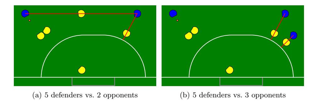
We illustrate the defense's coordination behavior when the play system of Section 2 has chosen the most defensive play, which has 5 robots assigned to defense. In this case, one defense robot is the goalie, 2 robots are PDs, and 2 are SDs; we illustrate the case in which both PDs are needed to guard $T_1$. Thus, only the behavior of the SDs varies as a function of the opponent's offense.
Two opponents: Figure 5a shows the positioning of a 5-robot defense against 2 offense opponents. Since there is only one $T_2$, the two SDs block the shot from and the pass to that threat.
Three or more opponents: Figure 5b shows the positioning of a 5-robot defense against 3 offense opponents. Our defense ranks shot-blocking tasks higher than pass-blocking tasks; thus, both SDs position to block shots from $T_2^1$ and $T_2^2$. If there are more than three opponents and hence more than two $T_2^i$, our algorithm ranks the $T_2^i$ based on the size $\phi$ of their shooting angle on the goal, ignoring robots, and our SDs mark the highest-ranked threats. If multiple robots have an angle φ larger than a threshold φ_max, they are ranked based on an estimate of the time t_goal it would take to complete a shot on our goal, where lower times are ranked higher. Time t_goal is calculated as t_goal = t_pass + t_deflect + t_kick, where
$$t_{\text{pass}} = \frac{d(\boldsymbol{x}b, \boldsymbol{x}T)}{v{\text{pass}}}, \quad t{\text{deflect}} = t_c \cdot \begin{cases} 0, & \theta \leq \theta_{\text{min}} \ 1, & \theta \geq \theta_{\text{max}} \end{cases}, \quad t_{\text{kick}} = \frac{d(\boldsymbol{x}_g, \boldsymbol{x}T)}{v{\text{kick}}}.$$
We estimate the time t_pass to pass to the threat using the distance d(x_b, x^T) between the ball location x^b and the threat location x^T, and the estimated opponent passing speed v_pass. We estimate the time t_deflect to deflect the ball to our goal based on the angle θ formed by x_b, x^T, and the goal center x_g: if a one-touch deflection is possible (i.e., θ ≤ θ_min), then t_deflect = 0; otherwise, t_deflect increases with θ, as defined by constants t^c and θ_max, estimated from the turning speed of the robots. Finally, we estimate the shot time t_kick similarly to t_pass, but using the opponent's shooting speed v_kick.
4.2 Contributions to Offense
RoboCup 2015 tournament introduced a new rule which prohibited players from entering either team's defense area. As a result, if a team's goalie has control of the ball inside its own team's defense area, it is safe from interference by the other team. We observed that this is effectively the chance to turn a shot on our goal into a free kick; to take advantage of this opportunity, we added the ability for the goalie to behave as a free kick taker under appropriate conditions.
The modularization of our code into tactics [9] enables the goalie tactic to simply use the tactic that takes actual free kicks; that tactic handles positioning and pass-ahead coordination with the receiver tactics. Although opportunities for the goalie to take this kind of kick were rare, there were two goals that we scored during the tournament as a direct result of these kicks.
5 RoboCup 2015 Results and Statistics
Our work on defense and offense coordination algorithms resulted in a dominant performance of the CMDragons at RoboCup 2015. The CMDragons played 6 official games during the tournament: three Round-Robin games (RR1, RR2, RR3), a Quarter Final (QF), a Semi-Final (SF) and the Final, winning all of the games by scoring 48 goals in total and conceding 0. Table 2 summarizes the offense statistics for shots and passes during each game.
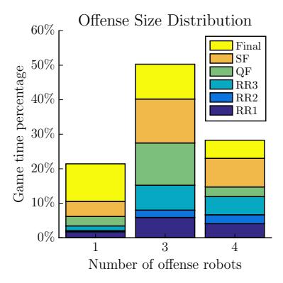
Persistent Offense: First, we highlight the highly offensive gameplay of the CMDragons. As Table 2 shows, our team attempted 148 shots on the opponent's goal throughout the tournament, successfully scoring on 48 opportunities. The CMDragons had an average shooting rate of 3.84 shots per minute of regular gameplay, and a scoring rate of 1.25 goals per minute. Figure 6a also demonstrates this highly offensive gameplay: our defensive play, which had only one robot in offense, was used only 21.4% of the time, while the rest of the time was devoted to more aggressive attack with 3 robots (50.3%) or 4 robots (28.3%). Figure 6b shows how this offensive gameplay enabled us to keep the ball mostly on the opponent's half of the field (66% of the time).
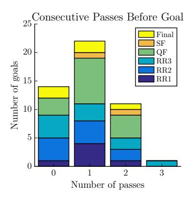
Team Coordination: Table 2 also highlights our team-oriented strategy, with 245 total attempted passes, of which 194 succeeded (79.2%). Per minute of regular gameplay, the CMDragons attempted 6.4 passes, and successfully completed 5 passes. Figure 7a shows that this team-oriented strategy played a crucial role in our gameplay: of our 48 goals, 22 were scored immediately after one successful pass, 11 goals after two successful consecutive passes, and 1 goal after three consecutive passes. Thus, team coordination enabled 34 of the 48 goals.
Regular Gameplay Performance: The team coordination algorithms described here shifted the focus of the CMDragons game toward regular gameplay intelligence, rather than stopped ball plays. Figure 7b shows the number of goals resulting from regular gameplay vs. those resulting from a stopped ball play. We define stopped ball goals as those that were scored either directly from our stopped ball or after a single pass, since our free kick planners (e.g., [10]) plan one-pass plays. The large majority of our goals were scored during regular gameplay. This distribution is in significant contrast with previous years: while only 56.7% of our recorded goals in RoboCup 2014 happened during regular gameplay, 79.2% of our goals in RoboCup 2015 happened during regular gameplay. We believe such shift of focus greatly benefited our team's performance in 2015.
Table 2: Statistics for each CMDragons game in RoboCup 2015. Games RR2 and RR3 ended early due to a Round-Robin 10-goal mercy rule, after 10:20 and 18:25 minutes respectively (normally, games last 20 minutes).
| Game | Shots Scored | Shots Missed | Shots Blocked | Shots Blocked (goalie) | Passes (other) rate (%) | Passes Attempts | Passes Success | Passes Missed | Passes Blocked | Passes Success rate (%) |
|---|---|---|---|---|---|---|---|---|---|---|
| RR1 | 6 | 2 | 4 | 5 | 35.3 | 32 | 2 | 7 | 78.1 | |
| RR2 | 10 | 2 | 2 | 1 | 66.7 | 14 | 4 | 0 | 77.8 | |
| RR3 | 10 | 3 | 5 | 7 | 40.0 | 30 | 5 | 2 | 81.1 | |
| QF | 15 | 8 | 5 | 12 | 37.5 | 38 | 2 | 2 | 90.5 | |
| SF | 2 | 3 | 6 | 20 | 6.5 | 51 | 6 | 6 | 81.0 | |
| Final | 5 | 2 | 6 | 7 | 25.0 | 29 | 7 | 8 | 65.9 | |
| Total | 48 | 20 | 28 | 52 | — | 194 | 28 | 23 | — | |
| Avg. | 8 | 3.3 | 4.7 | 8.7 | 32.4 | 32.3 | 4.7 | 3.8 | 79.2 |
6 Conclusion
Our coordination algorithms in offense and defense are largely responsible for the CMDragons' success at RoboCup 2015. This paper presents the algorithms for (a) assigning our robots to defense and offense subteams, and (b) creating coordinated plans for each subteam. In offense, we present a zone-based coordination algorithm that combines the benefits of planning independently of the opponents with those of appropriately reacting to them. In defense, we describe our threat evaluation algorithm to rank opponents as threats, and to assign defending robots to these threats. We show, via statistics from RoboCup 2015, that our coordination algorithms generated a persistent state of offense, effective teamwork, and a shift from stopped ball plays to regular gameplay. Our future work will focus on greater online autonomous adaptation to different opponents.
References
- M. Veloso, P. Stone, and K. Han. The CMUnited-97 robotic soccer team: Perception and multiagent control. Robotics and Autonomous Systems, 29 (2-3), 2000.
- M. Veloso, M. Bowling, and P. Stone. The CMUnited-98 champion small-robot team. Advanced Robotics, 13(8), 2000.
- J. Bruce, S. Zickler, M. Licitra, and M. Veloso. CMDragons: Dynamic Passing and Strategy on a Champion Robot Soccer Team. In Proceedings of ICRA, 2008.
- J. Biswas, J.P. Mendoza, D. Zhu, S. Klee, and M. Veloso. CMDragons 2014 Extended Team Description Paper. In RoboCup, 2014.
- J. Bruce and M. Veloso. Fast and accurate vision-based pattern detection and identification. In ICRA, pages 1277–1282, 2003.
- J. Bruce and M. Veloso. Real-time randomized path planning for robot navigation. In IROS, pages 2383–2388, 2002.
- S. Zickler and M. Veloso. Efficient physics-based planning: sampling search via non-deterministic tactics and skills. In AAMAS, pages 27–33, 2009.
- J. P. Mendoza, M. Veloso, and R. Simmons. Detecting and Correcting Model Anomalies in Subspaces of Robot Planning Domains. In AAMAS, 2015.
- B. Browning, J. Bruce, M. Bowling, and M. Veloso. STP: Skills, tactics, and plays for multi-robot control in adversarial environments. Proceedings of the IME, Part I: Journal of Systems and Control Engineering, 219(1):33–52, 2005.
- J. Biswas, J. P. Mendoza, D. Zhu, B. Choi, S. Klee, and M. Veloso. Opponentdriven planning and execution for pass, attack, and defense in a multi-robot soccer team. In AAMAS, 2014.
- M. Bowling, B. Browning, A. Chang, and M. Veloso. Plays as team plans for coordination and adaptation. In RoboCup 2003: Robot Soccer World Cup VII.
- J. P. Mendoza, J. Biswas, D. Zhu, R. Wang, P. Cooksey, S. Klee, and M. Veloso. CMDragons 2015 Extended Team Description Paper. In RoboCup, 2015.
- J. P. Mendoza, J. Biswas, P. Cooksey, R. Wang, D. Zhu, S. Klee, and M. Veloso. Selectively Reactive Coordination for a Team of Robot Soccer Champions. In Proceedings of AAAI-16, February 2016.
- D. Zhu, J. Biswas, and M. Veloso. AutoRef: Towards Real-Robot Soccer Complete Automated Refereeing. In RoboCup 2014: Robot World Cup XVIII.
- J. P. Mendoza, M. Veloso, and R. Simmons. Online Learning of Robot Soccer Free Kick Plans using a Bandit Approach. In ICAPS, to appear, 2016.