ER-Force Extended Team Description Paper RoboCup 2016
Christian Lobmeier, Peter Blank, Jonas Buehlmeyer, Daniel Burk, Michael Eischer, Adrian Hauck, Markus Hoffmann, Stefan Kronberger, Markus Lieret, Bjoern M. Eskofier
Digital Sports, Pattern Recognition Lab, Department of Computer Science Friedrich-Alexander University Erlangen-Nürnberg (FAU), Erlangen, Germany; Robotics Erlangen e.V., Martensstr. 3, 91058 Erlangen, Germany
http://www.robotics-erlangen.de/
Abstract This paper presents proceedings of ER-Force, the RoboCup Small Size League team from Erlangen located at Friedrich-Alexander-University Erlangen-Nürnberg, Germany. We present a curved kick bar to ensure a more straight shot. This is followed by our experiences with using a reflective break beam. A simple design for the robot's motion control is presented. Furthermore, we share our algorithm for calculating the time point at which the robot is able to catch the ball. It uses a twophase ball model to predict the ball's position and velocity.
1 Introduction
ER-Force has successfully partaken in RoboCup competitions for almost a decade. In this Extended Team Description Paper we would like to present our most recent efforts in improving both our hardware and software. We hope that our remarks support other teams in making Small-Size-League an even faster and more interesting league.
Our mechanical design has undergone improvement solely in the kicking system. Section 2 describes the aiming problems we had last year. A curved kick bar will ensure a straighter shot and, hopefully, lead to more scored goals.
Another problem we intend to solve is homemade: the general design of a reflective break beam detecting the presence of the ball from a central position inside the robot showed an unsatisfactory performance. Section 3 explains our experiences and suggestions on how to use such device successfully.
Section 4 introduces a simple design for the robot's motion control. This is complemented by an explanation of how to limit the motor current and hints for tuning the PID-controllers.
Finally, Section 5 re-evaluates a two-phase ball model first introduced by team FU-Fighters. Measurements conducted with our AutoRef software were used to validate the formulas describing the movement of a kicked ball, helping to predict ball position and velocity. This is complemented with an algorithm to estimate the time a robot needs to catch the ball. The topic is of particular importance with game moves increasingly relying on passing and intercepting rolling balls.
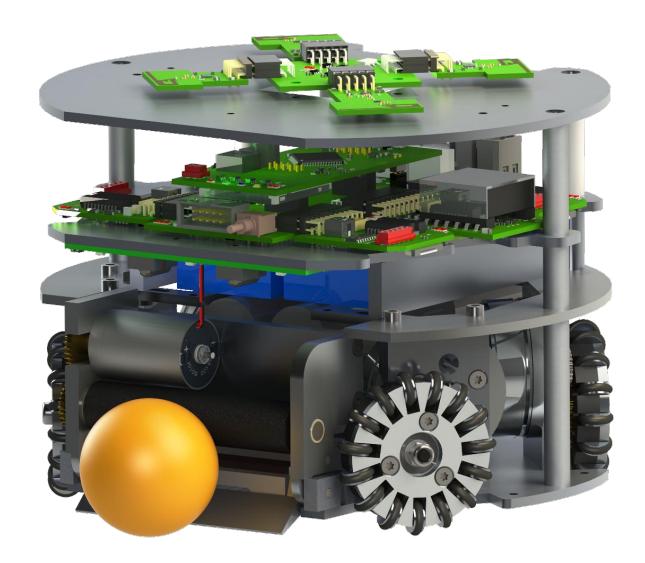
2 Mechanics
The current mechanical system is largely based on the design from 2014. See 2014's Team Description Paper [1] for details. A few modifications made to tackle performance issues are described below.
2.1 Dribbling Device
The tilting axis of our dribbling device was moved from vertically below the dribbling bar to horizontally behind the dribbling bar. Thus it can move slightly upwards when touching the ball. We hope that this approach will lead to reduced ball bouncing.
2.2 Kicking system
Chip kick A bar was added to the backside of the chip kick plunger to act as a physical stop. With this change the elastic band, which was used as a retraction and stopping mechanism, can no longer rip apart. Therefore, the plunger should now stay inside the robot.
Flat kick The kicking plate's shape of the flat kick was modified to improve precision and reliability. Our flat kick consists of a divided plunger rod, which is connected to the kicking plate. The plunger rod is guided inside the coil body and additionally, the kicking plate is guided by two linear sliding guides. Due to jamming of the flat kick, when coil and sliding guides are misaligned, the sliding guides were adjusted to a loose fit.
During the last RoboCup event our robots did not kick in the expected direction in some situations.
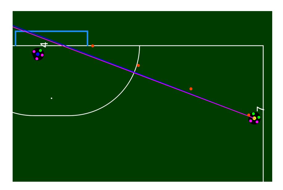
In figure 1 a corner kick situation in the group stage game ER-Force in yellow vs. NEUIslanders in blue is shown. The ball trajectory is indicated by the orange balls. The blue line indicates the current direction our robot is facing, along with the intended kicking direction in pink. Obviously the ball trajectory differs significantly from the direction our robot is facing. This happens because the kicking robot is not perfectly centered behind the ball and thus is hitting the ball at an off-center position.
The resulting force affecting the flat kick can be described as a linear force acting at the center axis and an additional torque. This leads to elastic bending of the linear plunger assembly. The kicking plate no longer hits the ball perpendicular to the kicking direction.
Tests were carried out to determine the deviation from the expected kicking direction based on where a ball was positioned in front of the dribbling bar.
The ball was placed at the center position and at 1, 2 and 3 centimeters to the left and right. The measured kicking angle for every position was averaged over 5 kicks resulting in table 1.
Table 1. Measurement results of the kick direction analysis
| position in cm | angular deviation in deg |
|---|---|
| -3 | -12.2 |
| -2 | -10.5 |
| -1 | -5.6 |
| 0 | 0 |
| 1 | 5.75 |
| 2 | 10.2 |
| 3 | 12 |
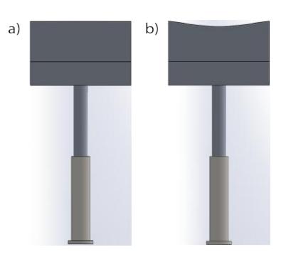
With this information a concave shape for the kicking plate was calculated to compensate the angle deviation of all possible ball trajectories.
The concave shape was calculated using the following approach. The shape of the kicking plate must be parabolic and the angle of the slope of this parabola must be equal to the angle $\alpha(x)$ by which the ball trajectory deviates from the expected direction. As stated, this angle depends on the lateral displacement $x$ of the ball towards the center of the dribbling bar.
Both parameters $\alpha(x)$ and $x$ can be measured. The slope of a parabola is described by its first derivation, thus the required shape of the kicking plate can be described as
$$f(x) = a(x) * x^2 \tag{1}$$
where $a(x)$ can be calculated as
$$a(x) = \frac{\tan \alpha(x)}{2x} \tag{2}$$
By interpolating our measured values $\alpha(x)$ we were able to calculate the new shape of the kicking plate and manufacture the prototype shown in figure 2 below.
3 Detecting the ball
This section describes our experiences with the reflective ball detection system introduced in 2014. It concerns only systems which are located above the dribbler on the robot to recognize the presence of the ball in a game.
For RoboCup 2014 team ER-Force tried a new method of ball detection. This was the first time the conventional linear light barrier system was replaced because of space issues within the robot. In difference to previous years a reflective light barrier was proposed and developed. The principle and all used parts are described in [2].
After two years of optimization and reengineering of this light barrier systems, we found that the reflective approach is not practicable. The poor results by this system have their roots in two main problems which could not be solved by our team so far.
The varying reflectance over the width of the dribbler poses a challenge which impedes the calibration of the light barrier. The construction of our dribbling system is not symmetrical because of the dribbler motor. It is shorter than the width of kicking system and overlaps only the half of the dribbler breadth. With the above mounted LEDs the amount of reflected light on the motors side is significantly higher than on the opposite side. Thus, a very protracted calibrating process is necessary to achieve an equal illumination over the whole width with fitted LED light levels. The practical implementation requires a manual adaption of three resistors.
The unequal reflectance of different balls was the second issue which occurred with the reflective system. Each golf ball behaves differently under the influence of infrared light. The amount of reflected luminous power differs from ball to ball and within one ball as soon as the orientation changes. Therefore, the calibrated threshold for firing a kick is always a compromise. In most cases, the evaluation of the correct threshold was more successful by chance than by doing exact measurements.
Our conclusion is that a reflective light barrier system does not work in the SSL environment. There are too many parameters that vary with the individual robots and golf balls. We suggest a combined approach: use a linear light barrier to detect the presence of the ball, and a reflective system to determine the ball position. However, for this RoboCup we will only use a linear light barrier.
For the limited purpose of kicking the ball in the correct moment with a high recognition quote, ER-Force is going to implement a linear light barrier system in the robot. The electrical circuit will stay the one described in last years ETDP [2]. Transmitter and receiver will be replaced with smaller parts. So these parts can be rearranged and placed in front of the kicking system. We are looking forward to achieving satisfactory results in 2016.
4 Motion control
Because our robot's motion control has been nearly unchanged for the last years, there is a lack of in-depth knowledge for its design in the current team. In addition, the orientation control was not reliable enough and the velocity control did not always reach the target speed. So we decided to redesign the motion control on the robot from scratch.
4.1 Design of our new motion control
The basic idea is to start with a system that is as simple as possible. For this reason we use PID-controllers, which are easy and fast to implement. They are based on measurements of the real system instead of theoretic models and are very robust against small mistakes in the parameters, which may be caused by inaccurate measurements.
Depending on the required time to implement, and the success of this controller, we consider adding a feedforward and replacing parts of the controller by more complex models for being able to compute and control non-linear correlations.
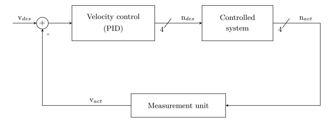
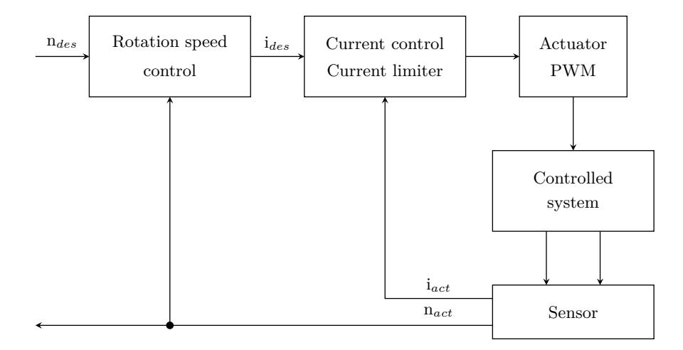
Due to our robots' design, the controller is split between the main board and the motor boards. The first part controls the robot velocity and is located on the main board. The second part runs on the motor boards, one for each wheel, and controls the rotation speed and current of each motor.
The first part is shown in figure 3. Using the radio modules it receives the desired velocity $v_{des}$ from the AI. The controller gets the desired velocity as input and computes the rotation speed for each wheel. These are calculated from the velocity output of the controller using the transformation described in [3]. The motor boards send their measured rotation speeds to the main board. The difference between the desired and the actual speed becomes the new input for the controller.
The second part placed in the motor boards is cascaded as shown in figure 4. The inner loop controls the motor current, while the outer loop controls the rotation speed of the motors. Each controller works with the same principle as the velocity controller. This means that simple and robust PID-controller are used.
The only exception in the controller design can be found in the most inner part of the controller, when controlling the current, because there is a limit implemented to protect the motor against overheating. For the moment, this limit is the highest current a motor can withstand for an extended period of time. The limiting is done by averaging the current over a time span of approximately ten seconds. On each run of the control loop, during which the average current exceeds 1.3A, the PWM limit is set to the last PWM value minus one percent. That is, the PWM value is repeatedly decreased until it compiles with the current limit. Once the average current falls again below the limit, the PWM limit will slowly be raised again. This shows potential for optimization, for example in accepted current peaks, but for the moment we prefer a robust system to an optimized but possibly critical system. In fact, this limiting scheme has successfully prevented any motors from overheating for two RoboCup events.
Potential for optimization can be found in the actuator as well. The actuator shall convert the desired theoretical current into a physical current. This means, that the desired current is converted to a duty cycle for the PWM. This conversion is highly non-linear and depends on many different values, mainly on the induced voltage inside the motors.
For the moment, a linear factor is used. The long term plan is to implement an inverse motor model. The advantage is that we can focus on the controller, while the disadvantage is a more challenging controlling behavior.
4.2 How to tune the PID-controller
While it is very easy to implement a PID-controller, there are different ways to create the parameters. We have chosen to derive them using the method of Ziegler-Nichols.
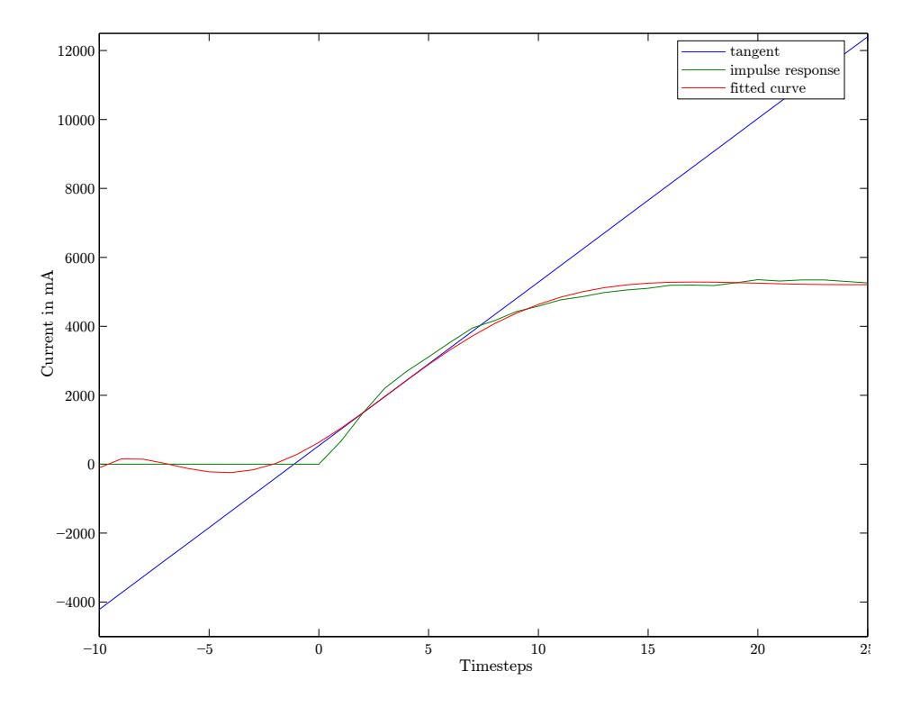
In order to do this, we apply an impulse on the uncontrolled system. The system is assumed to react in a way which can be approximated as a PT2 behavior. The reaction has to be measured and added to a graph as shown in figure 5. This graph is used to synthesize the PID-parameters. For this an inflectional tangent has to be calculated and added to the graph. The time from the beginning of the impulse till the intersection of the tangent with the x-axis is called $T_u$, whereas the time from the intersection with the x-axis till the intersection of the tangent with the maximum is called $T_g$. These are the important time-constants. Further, you have to calculate a proportional value. This value called $K^s$ is calculated by dividing the actual maximum by the desired maximum.
$$K_s = \frac{max_{act}}{max_{des}} \tag{3}$$
In the graph for example there is a desired maximum of 5000 and an actual maximum of approximately 5000, so that $K^s \approx 1$.
As soon as these three values are known, the PID-parameters can be calculated using the following formulas:
$$K_P = \frac{1.2}{K_s} \frac{T_g}{T_u} \tag{4}$$
$$K_I = \frac{K_P}{2T_u} \tag{5}$$
$$K_D = K_P \frac{T_u}{2} \tag{6}$$
It is important to be aware that these parameters are just an initial estimation. Although this is a systematic way to create parameters there will for sure be potential for optimization, thus it is recommended to modify the parameters afterwards for better results.
In addition, the D-parameter of the PID-controller for the current should be set to zero or at least smaller than on the other PID-controllers, because depending on the quality of the measuring unit a large D-parameter can lead to destabilization.
5 Two phase ball model
5.1 Ball model
Prior to last year's RoboCup event, we used a very simple approximation for the ball physics: The velocity of the ball decreases with a constant deceleration until the ball reaches a resting state. Even though this model seems evident in the first place, it does not fit our observations of a real ball.
One other possible model would be to use a polynomial fit as in [4] or [5]. It was shown to yield a better approximation of the ball movement.
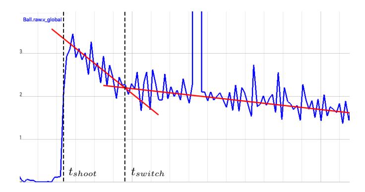
As our previous ball model had not provided satisfying results, we readdressed this issue using a simple physical model. The ball, which has a velocity and angular momentum, is modeled as a sphere rolling over the ground. At $t_{shoot}$ the ball has a very high forward momentum whereas its angular momentum is close to zero. Thus, the ball slides over the ground and a substantial amount of the energy is transformed into rotational momentum. The exact amount of energy is determined by the rolling friction. Starting at $t_{switch}$, the ball rotates as fast as it moves forward - it rolls. Therefore, the deceleration is much lower. In fact, the only force that slows down the ball is its friction which generates a velocity independent force that slows down the ball. The described forces are constant as long as they apply, thus causing a constant deceleration of the ball.
This yields the two phase ball model as described by FU-Fighters [6].
Figure 6 shows the velocity of a ball which was shot at 3.3 m/s. The graph shows that the two phase ball model matches the measured data very well. Due to these promising results we assume that this model is more accurate than using a polynomial fit. However, we did not conduct detailed tests.
5.2 Parameters
The exact time points and decelerations are contingent on the playing field. To predict the ball's movement, one has to know the current ball speed $v_{current}$, the decelerations $a_{slide}$ and $a_{roll}$ and the time $t_{switch}$.
- The velocity of the ball $v_{current}$ is always known.
- One can assume that the decelerations $a_{slide}$ and $a_{roll}$ are constant. Using our plotter software, we measured $a_{slide} = -2.5 \frac{m}{s}$ and $a_{roll} = -0.3 \frac{m}{s}$.
- According to FU-Fighters, the ball speed $v_{switch}$ at the time $t_{switch}$ is proportional to the initial shoot speed $v_{shoot}$. In theory, the ratio between $v_{switch}$ and $v_{shoot}$ is $c_{switch} = \frac{5}{7}$. However, our tests suggest a value of $c_{switch} = 0.6$. Using this estimation, the corresponding time point can be calculated with the following formula (assuming $t_{current} = 0$):
$$t_{switch} = \frac{v_{switch} - v_{current}}{a_{slide}} = \frac{c_{switch} \cdot v_{shoot} - v_{current}}{a_{slide}}$$
To implement this two phase ball model, the initial shoot speed $v_{shoot}$ has to be tracked. In general, $v_{shoot}$ has to be updated when the ball speed increases.
5.3 Ricochets
However, this ball model can lead to incorrect predictions after the ball ricochets because it usually changes its state to sliding without actually being shot. A naive approach would be to also update $v_{shoot}$ if the ball changes its direction.
While this might work if the ball's direction after the ricochet is roughly perpendicular to its original direction, the remaining rotational energy of the ball will influence the ratio between $v_{switch}$ and $v_{shoot}$. With the ratio $c_{switch}$ no longer being constant, acquiring viable parameters requires a lot more testing.
Another problem is, that after ricochets, the ball will most likely travel in an arc-like shape which makes a fast and solid prediction close to impossible. Therefore, our implementation completely ignores ricochets.
5.4 Calculating the ball roll time
The actual algorithm for computing the time the ball needs to travel a given distance d is quite straightforward.
Algorithm 1 ballRollTime(ball, d)
if v_{current} < v_{switch} then
  solve for t in 1/2 · a_{roll} · t^2 + v_{current} · t - d = 0
  return t
end if
t_{switch} ← (v_{switch} - v_{current})/a_{slide}
d_{switch} ← 1/2 · a_{slide} · t_{switch}^2 + v_{current} · t_{switch}
if d < d_{switch} then
  solve for t in 1/2 · a_{slide} · t^2 + v_{current} · t - d = 0
  return t
end if
solve for t in 1/2 · a_{roll} · t^2 + v_{current} · t - (d - d_{switch}) = 0
return t + t_{switch}
- First, the speed $v_{switch}$ at which the ball transitions from sliding to rolling is computed.
- If the ball is already rolling, calculate the time it needs to travel the given distance using the deceleration $a_{roll}$.
- Otherwise, compute the time and the distance the ball needs to reach $v_{switch}$.
- If the given distance d is smaller, calculate the time using the deceleration $a_{slide}$.
- If not, the ball has a slide and a roll component. In that case, calculate the time of the latter one and add it on top of the previously computed slide time
With the aid of a similarly structured function, the ball position at any given time can be predicted.
5.5 Predicting the robot to ball time
One of the most interesting questions in robot soccer is how long it takes a robot to reach the ball. We introduce a procedure based on the estimation function robotTimeToPos as a black box as well as on functions using the previously presented two phase ball model.
Consider the following situation:
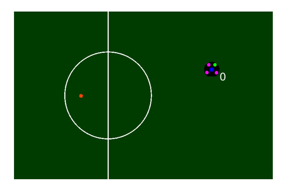
- Initially, the robot is standing still
- The ball rolls to the right at 2.0 m/s
- The robot wants to catch the ball while facing to the left
- The robot and the ball are positioned as shown in Fig. 7
The goal is to find the first moment in which the robot can touch the ball with the dribbler while facing in the desired direction. More formally, we are interested in the smallest time $t_{ball}$ where
$$t_{robot}(t_{ball}) < t_{ball}$$
with $t_{robot}(t_{ball}) = \text{robotTimeToPos}(ballAtTime(t_{ball}) - offset)$. The vector offset is used to model the fact that the robot catches the ball with its dribbler not its midpoint. Therefore, it is the vector having the distance between midpoints of the ball and robot when touching the ball and points towards the robots intended target.
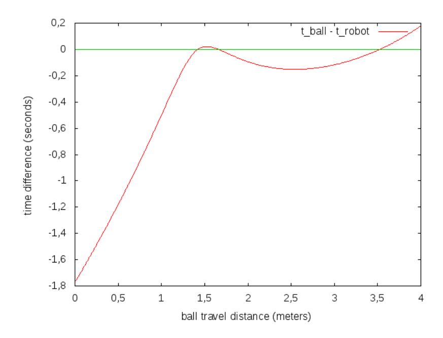
Figure 8 shows the difference between those two times relative to the distance the ball has to travel. Because the relation between $t_{ball}$ and this distance is strictly monotonical, the first catch point in time is also the leftmost one in the graph.
This graph shows that there is a small window of roughly 0.25 m where the robot is fast enough and can catch the ball by directly moving in its way. Another option is to get the ball when it is slow enough for the robot to catch up. In this example, that will happen at about 3.5 m. The first interval does not always exist, as well as the first peak in the graph. However, it is guaranteed that there is at least one point where the robot can catch up to the ball. In the worst case, the ball has already stopped when the robot arrives. This position is more often than not outside the playing field.
Because the ball functions consist of multiple partially defined functions and especially because robotTimeToPos is considered a black box, the first catch point cannot be computed directly. Instead, we use two loops to get an acceptable result without spending too much compute time.
The required time to stop the ball is calculated by algorithm 2. The upper bound for the sampling consists of $t_{stop}$ (the time the ball needs to come to a stop) and $t_{out}$ (the time until the ball will cross a border of the field), thus this procedure cannot find catch points outside of the field.
Algorithm 2 robotTimeToBall(robot, ball, targetpos)
tmax ← min(tstop, tout)
for ti in range [0, tmax] do
  if (ti, ti+1) satisfies trobot(ti) ≥ ti and trobot(ti+1) < ti+1 then
     in this interval, do a binary search for trobot(t) = t
     return t
  end if
end for
return (tstop < tout) ? trobot(tstop) : ∞
The first sampling loop searches for an interval where the corresponding time difference graph crosses the zero from the negative to the positive space. The granularity of the sampling determines whether a small first interval will be detected each frame or not.
If such an interval is found, use a binary search to find the desired time point with an appropriate accuracy. In general, this approach only works if the underlying function is steady. Actually, when the robot moves towards the ball, the graph shows a discontinuity. The discontinuity emerges because the robot can reach its current position in zero seconds while it takes the robot a considerable amount of time to get back to a position right behind its current one. Because of this, the binary search has to be limited by the number of iterations instead of the quality of the result.
If no suitable interval was found in the first place, the robot cannot reach the ball until it stops or rolls out of the field. Depending on which event happens first, a meaningful time is returned.
6 Conclusion
In this paper, we aimed at sharing the lessons learned from our past mistakes in Mechanics, Section 2 and Electronics, Section 3. We also intended to provide information for improving software in Motion Control, Section 4 and Strategy, Section 5. We hope that these topics represent valuable input for teams working in these fields.
Some topics have been developed further based on previous Team Description Papers. Likewise, we look forward to hearing other teams' comments.
References
- Bayerlein, H., Danzer, A., Eischer, M., Hauck, A., Hoffmann, M., Kallwies, P., Lieret, M.: Team Description Paper for RoboCup 2014 (2014)
- Eischer, M., Blank, P., Danzer, A., Hauck, A., Hoffmann, M., Reck, B., Eskofier, B.M.: Team Description Paper for RoboCup 2015 (2015)
- Rojas, R.: Omnidirectional control. (2005)
- Ryll, A., Ommer, N., Geiger, M., Theis, J., Bayer, F.: TIGERS Mannheim (Team Interacting and Game Evolving Robots) Extended Team Description for RoboCup 2015 (2015)
- Rodríguez, S., Rojas, E., Pérez, K., López, J., Quintero, C., Calderón, J.M., Peña, O.: STOx's 2015 Extended Team Description Paper (2015)
- Rojas, R., Simon, M.: Like a rolling ball. http://robocup.mi.fu-berlin.de/buch/rolling.pdf retrieved 19 January 2016.