KIKS 2016 Team Description
Tatsuro Sakaguchi, Koh Ohno, Toshiki Mimura, Naoki Tanaka, Kenta Satoh, Yu Yamauchi, Yoshimasa Nagasaka, Masato Watanabe, Toko Sugiura
National Institute of Technology, Toyota College, 2-1 Eisei-cho, Toyota Aichi, 471-8525, Japan
http://www.ee.toyota-ct.ac.jp/~sugi/RoboCup.html
Abstract This paper is used to qualify as participation to the RoboCup 2016 small size league. Our team's robots and systems are designed under the RoboCup 2016 rules. The major points of improvement in this year are about the kick bar, motor unit, electrical circuit and AI system. The overviews of them are described.
1 Introduction
KIKS mainly consisted of students' age 21 and younger that has been competing at RoboCup since 2002. In RoboCup last year, we had bad performance in both of Japan open and world competition. The main reason is that the technical know-how is not handed down from elders to new students in sufficient, and also related to a decrease in membership. In this coming competition, we would like to approach the game as new-comer restudying all over from the basics.
We still have many problems with a kinematic, an electrical circuit and strategy performance of robots. In order to solve these problems, we attempted to improve our robots in 2015 [1]. It is described as the terms of the mechanical, electrical and electronic, software as follows.
2 Mechanical improvements
Our robots are equipped for two type of kicking devices, dribbling device and other minimum functions based on the rule of SSL. But, these equipment do not play enough role during the game. Now, we can say that serious problems are belong to straightness of kicked ball and running stability of the robots.
2.1 Improvement for kick device
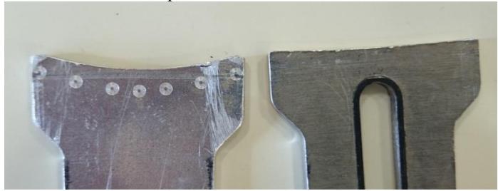
About the term of straightness related kick devices, we tried to change the kick bar that has the shape like a parabola. As the results, this shape gave us the good suppression efficiency for variability of ball's direction. Figure 1 shows new shape of kick bar (left) including old one (right). We evaluated about straightness of kicked ball. The ball was kicked to the destination located 1m away from robot. In previous kick bar, it found that the standard deviation of arrived positon of ball is 5mm over, while new curved bar was less than 0.5mm. It means, that is, 10 times better than previous one. Moreover, that performance is depending on not only shape but also material. It was found that plastic bar shows better trend, if compared with metal bar. So, we will introduce this new kick bar, after the detailed evaluation of performance about durability and other factors between plastic bar and metal one.
2.2 Improvement of related motor unit structures
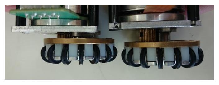
We made efforts to simplify manufacture the motor unit. Up to now, we had need to make screw hole on the gear, and tighten screw to connect with motor axis. In new method, the gear is simply connected with motor axis using dual liquid adhesive agent. We examined the applicability of that method on terms of strength. As the results, there is no problem, and it helps us to design thinner motor unit, as shown in Fig. 2. It was possible to thin about 6mm.
On the benefits of thinning motor units, we can design and arrange flexibly equipment such as solenoids or dribbling devices with less limitation because inside space of the robot might have larger volume.
2.3 Trial to introduce 70 Watt motors
We tried to introduce 70 Watt motor to enhance the motion performance of robot.
Trial a mechanical term
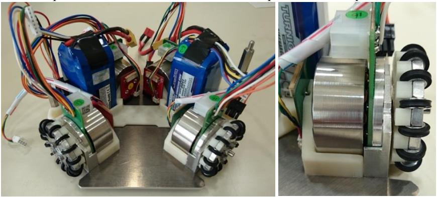
Maxon EC45 flat 30Watt motor (200142) is now used in our robot with 18:60 reduction ratio. In this case, maximum torque is 750mNm and maximum speed of the robot is 3.4m/s theoretically under the condition of no load. While the case of maxon EC45 flat 70 Watt motor (402687) will be used, and motor's torque will be 915mNm. This is, 70Watt motor's torque is 1.2 times stronger than present one. It suggest that use of the 70Watt motor can be used without any reduction system. Moreover, we expect to be faster robot because maxim speed of the robot with 70watt motor is prospected to be around 9m/s under the condition of no load. The test-robot with maxon 70Watt motors and 70Watt motor unit are shown in Fig. 3. Furthermore, this 70Watt motor unit is designed as thin as 30 Watt motor unit, because there is no need to use reduction gears.
We have not done enough quantitative evaluation yet, but stability and acceleration of the robot have become better on qualitative viewpoint. So, we will test continuously about the performance of this robot and make a replacement from present robot.
Improvement of circuit for 70Watt motor
We tried to make an attempt of the circuit for implementing 70Watt motor. In that case, it will be need to use two 6cell Li-Po batteries. Previously, however, our main circuit board (which can manage communications and control motor driver) can only apply up to 25V. So, the improvements were required applying to until 50V. Then, we designed it not connecting to kicker board (which can charge and manage the capacitor, and operate switching device called IGBT when it get kick-command).
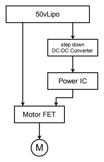
Current main board is worked on a 4cell Li-Po battery, so it is designed under the maximum voltage of 17V. And DC-DC converter IC, which apply to four kinds of voltage now we are using, can give us only until 40V. We could not find any IC applicable for 50V to replace old IC. So we tried to redesign a circuit to step down the voltage for power IC and to connect directly for motor FET as shown in Fig. 4.
We had to evaluate and decide as soon as possible about the use of the 70Watt motor. We do not have much time to verify as our finished circuit. So, we adopted the way as making extension sub-board and mounted on the main circuit board. The power line which comes from Li-Po Battery is distributed to the Motor Driver IC and DC-DC converter. Then it steps down to 15V from 50V the voltage through DC-DC converter 50V and output 15V. In addition, for the capacitor and diode, it was replaced to applicable equipment working on 50V power line.
3 Electrical improvements
3.1 Trial a use of SoC FPGA
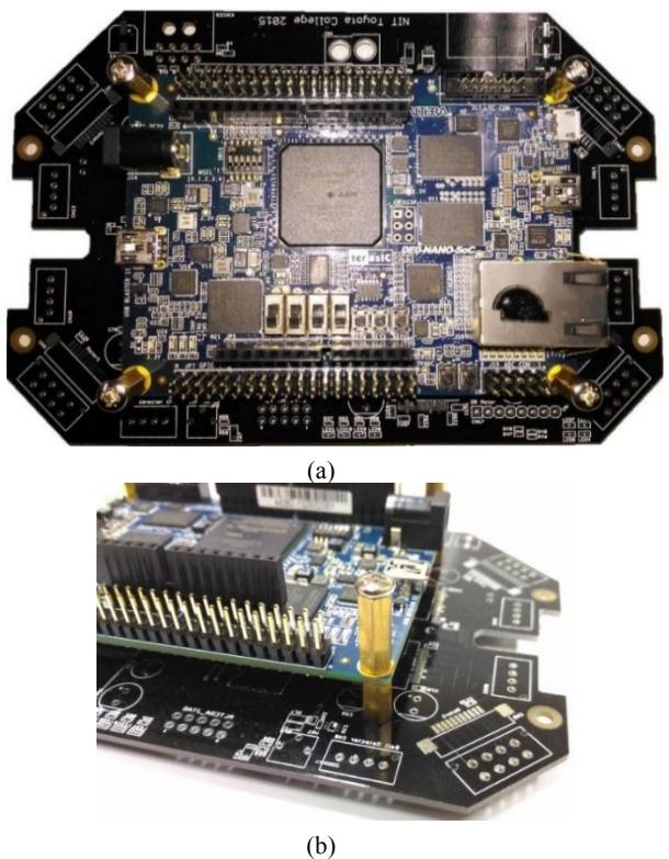
Right now, our electronic circuits are working well without any problems. We can confirm the wheel speed for each robot, ball sensor status through Windows computer via USB. Each robot controls four motor by sending data from AI computer during the game. In this year, we tried to make an improvement to replace from the function of AI to that of robot partly. It was examined by using SoC FPGA. To introduce SoC FPGA, we renewed a circuit as shown in Fig. 5. DE0-Nano-SoC placed in center of the renewal circuit has ARM CortexA9. Linux OS supplied as the FPGA vender is able to run on the CPU.
In our FPGA, it has two 40-pin expansion headers. The header-drivers include the BLDC motors, sensors, communication-devices, and so on. DE0-Nano-SoC also has ADC (Analog Digital Convertor) which can get battery voltage. Hardware on FPGA can be controlled by ARM running on Linux via FPGA-ARM bridge, if we need. Now, it was finished on the point of controlling four BLDC motors. It is remained as future research that it makes the connection between AI and the board via wireless communication and motor-control. The board will supply much resource to calculate faster.
3.2 Role of AVR
Communication and processing on AVR
An AVR has a function of transition via USB on a physical layer. We can use "Terminal" developed to write only on logics and each of firmware on FPGA through AVR. In working of FPGA, it is getting several information on a queue and AVR also has a role which send information from queue to "Terminal".
Management for battery
An AVR have an ADC connected with a battery. The battery level corresponding to three statuses is displayed as the color of LEDs to lead us to understand visually. A final voltage of Li-Po battery is 3.3V. Therefore, when a voltage of cells on a battery downs to 3.3V, the process is finished and the power are shut down for protection.
Programing on FPGA
Spartan-6 which use for motor controls is a volatile FPGA. Thus, if it is shut down the power, the structure information of FPGA is vanished. We must write to FPGA as an initialization. An AVR connects to writable pins on FPGA to programs to one form a nonvolatile memory (EEPROM) at starting process. Also an openMSP430 Core working on FPGA is written at the same time because of same reason.
3.3 Control for circuit
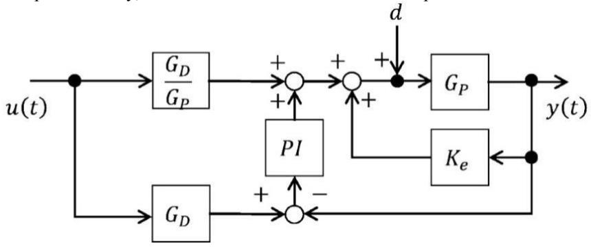
Motor control is performed by the angular velocity in the FPGA. Two degree of freedom PI control system is used to improve following performance to target value and performance of disturbance control. Block diagram of control circuit is shown in Fig. 6. The ultimate gain method are used to calculate the proportional gain and integral gain. Ke is given as fixed number of counter electromotive force. Gp, that is, transfer function model of motor is tentatively adopted 1, because it did not work well in our experimental stage. So, it is assuming that there is no delay and loss to the input and output. Similarly, Gd related factor of feed forward compensation is set as 1.
4 Improvement of the AI system
4.1 New AI System
Recently in RoboCup SSL, in addition to the simple control of the robots, it has an ongoing effort to analyze log data of the game and use for tactics by some teams. In our AI, however, it is very difficult to do that. Because technical know-how is not sufficiently handed down from elders to new students. In addition, the maintenance and development for strategy have not fully been continued. So, we decided to rebuild the next AI system in parallel with the improvement of present system. The concept of this project and the present situation are described below.
Design
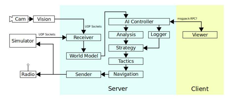
It is expected that PC has high performance for the analysis of data. However, it is difficult that all developers have such PC. Thus, we examined to divide into the server- and client- parts as shown in Fig. 7.
Server
One independent PC that has enough performance executes as server of AI system. It connects to a Client by RPC protocols like messagepack-rpc [2] and executes the program of each strategic part in accordance with an order from a client. In addition, the new module is implemented to record and analyze for the log data of games. It is not prepared these functions in present system.
Client
It is executed by developers' own computers. It sends the orders of choice and execution of the strategic program and the change of the parameter to a server. In addition, it show the game situation based on the information provide from a server.
In present situation, the parts related strategy and communication to the robot does not sufficiently achieve yet. Other parts are mostly finished. Now, we are implementing the strategic part to play in the game next coming Japan Open 2016. We have a plan to analyze the game-log mainly hereafter.
4.2 Field analysis for passing
In recent year, the offence play using some passes a ball become more and more mainstream. The passes must be succeeded to get scores. However, the defense play is also getting better in all teams, therefore simple passes tends to fail. We have faced the serious problem with pass for attacking, and it causes the loss of chance to get scores. Thus, we made two programs dynamically finding the passing course for a ball. One is using circles to help an instinctive feel, and the other is using tentative score corresponding to the position of the opponent robots and other field circumstance.
Selection using circles
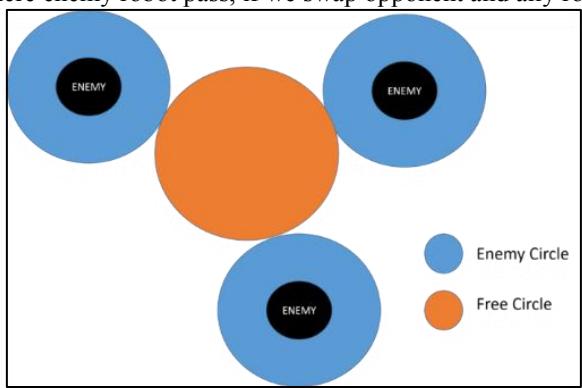
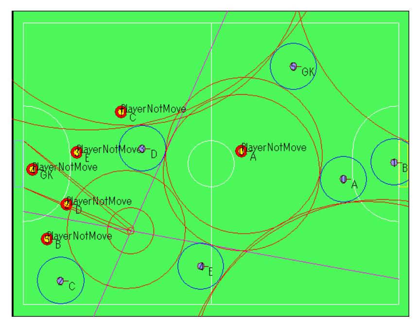
We make circles which show the area enemy's robot can move. The radiuses of these circles are input by users. These circles are defined as Enemy Circle, and the circle space where enclosed by three points in contact with outer of Enemy Circle is defined as Free Circle. These circles are shown in Fig. 8. It is obtained that pass course from the circumscribed line of Enemy Circles and Free Circles. Figure 9 shows the typical results displayed on simulator for pass courses.
Blue and red circles show the Enemy and Free Circles, respectively. Pink lines mean possible pass courses. If we do not want to pass to own penalty area, we can find the pass-prohibited area. The passing course may include an angle which we want. So we can set limit value against the angle to allow the pass. Furthermore, learning functions are able to add to this system. For example, radius of Enemy Circle is possible to change based on the information for the time spent on passing and enemy robot's speed. Enemy Circle is also changed into an oval, if danger areas are spread out depending on the velocities of enemies. In addition, we can make a prediction the area where enemy robot pass, if we swap opponent and ally robots.
Selection by scoring
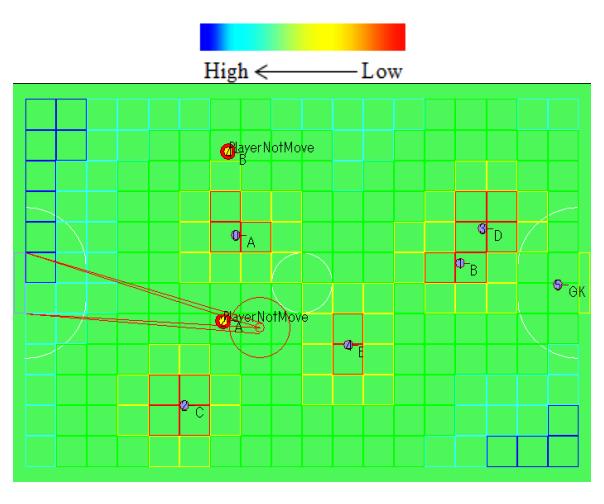
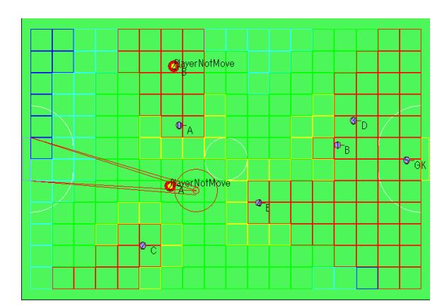
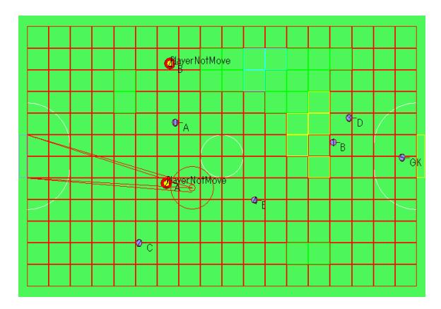
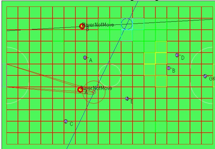
In Fig.10, the game field is divided into grids with 500mm x 500mm area and each of them is assessed as candidates of pass target. Then, each grid has score which is used when the passing target of ball is decided. We gave the scores for grids in accordance with six rules described (A) - (F) as follows.
- (A) Farthest grid part from an opponent robot, the higher score is given.
- (B) Grid located in the direction which opponent robots go, the lower score is given.
- (C) Grid located in the back side of opponent robots and ball, the lower score is given.
- (D) Grid located in the penalty area, the lowest score is given.
- (E) Grid located in close to a ball, the lower score is given.
- (F) Grid located in the direction for attacking area, the higher score is given.
Figure 10-13 show the colored grid with different color based on the condition as mentioned above. The rule (A), (B) and (C) are indicated in Fig.10 and 11, and the rule (D), (E) and (F) are indicated in Fig.12, respectively. These figures are classified by the color bar shown in below.
4.3 Path finding to avoid collision
It is required to avoid collision between robots in RoboCup Small Size League, because of the importance to prevent from damage of robots. Right now, many teams adopt the RRT (Rapidly exploring Random Tree) algorithm to avoid collision [5]. Our team also applies to it. But, the RRT algorithm needs a large amount of calculation and the computed paths are complicated for us. Other teams have introduced using a GPGPU(General-purpose computing on graphics processing units) or an improved RRT algorithm, but we do not think absolute necessary to spend much time to calculate path finding, and not also think proper to search the path individually because ally robots can share mutual information. So, we tried to introduce ORCA (Optimal Reciprocal Collision Avoidance) algorithm as multi-agent system which needs less amount of calculation for application to SSL.
ORCA algorithm
ORCA algorithm calculates a velocity region where robots A and B collide during the prediction time $\tau$ and let us know the information that does not select its region [6]. It also makes a calculation of the region between the robot A and all robots near the robot A, it results where a robot A moves.
A velocity region where collision occurs.
Let relative position $p_{AB}$ be defined as $p_{AB} = p_B - p_A$, where $p_A, p_B$ are the coordinates of the robots A and B, respectively and the radius $r_{AB}$ as $r_{AB} = r_A + r_B$, where $r_A, r_B$ are the radius of robots. Then, the region within the radius of $r_{AB}$ from the center $p_{AB}$ is inside a circle where collision occurs. If the collision region in prediction time $\tau$ is taken into account, $p_{AB}(t)$ and $r_{AB}(t)$ are as follows.
$$P_{AB}(t) = \frac{p_{AB}}{t}(0 < t < \tau)$$
$$r_{AB}(t) = \frac{r_{AB}}{t}(0 < t < \tau)$$
A velocity region $VO_{AB}^t$ which robots collide is inside a circle with the radius of $r_{AB}(t)$ and the center $P_{AB}(t)$.
Selection of velocity.
The robot B gives the half-plane limit region to robot A by the ORCA line drawn from the $VO_{AB}^t$ and the other robots near the robot A also does. Then, the $V_A^{new}$, which is likely to match the preferable velocity $V_A^{pref}$ of the robot A, is computed by using linear programming as the limit speed of maximum $V_A^{max}[7]$.
Improvement of ORCA algorithm
The algorithm mentioned above section does not consider for acceleration, so it is not suitable for the situation that change the velocity instantly. In the RoboCup SSL, the robots move freely with maximum speed of about 3m/s and maximum acceleration of about 2m/s² at a refresh period of 1/60s. So it is required to take into account the acceleration and control the robots to avoid collision.
Firstly, if it considers the acceleration, the velocity gradually changes over time, so the center c(t) and the radius r(t) of a circle of the velocity region which collision occurs are as follows [8].
$$c(t) = \frac{\delta\left(e^{-\frac{t}{\delta}}-1\right)v_{AB}-p_{AB}}{t+\delta\left(e^{-\frac{t}{\delta}}-1\right)} (0 < t < \tau)$$
$$r(t) = \frac{r_{AB}}{t+\delta\left(e^{-\frac{t}{\delta}}-1\right)} (0 < t < \tau)$$
Here, $\delta$ is defined as a proportional control parameter of acceleration and relative position $p_{AB}$ and relative velocity $v_{AB}$ being used in formula (3),(4) are as follows.
$$p_{AB} = p_A - p_B$$
$$v_{AB} = v_A - v_B$$
The ORCA line is drawn by using the velocity region of a circle with the center c(t) and the radius r(t). Then, linear programming with the center value of the current velocity $v_A$ is performed under the condition of limit acceleration $\delta a_A^{max}$ ($a_A^{max}$ is the maximum acceleration).
Avoidance simulation using 4 Robots
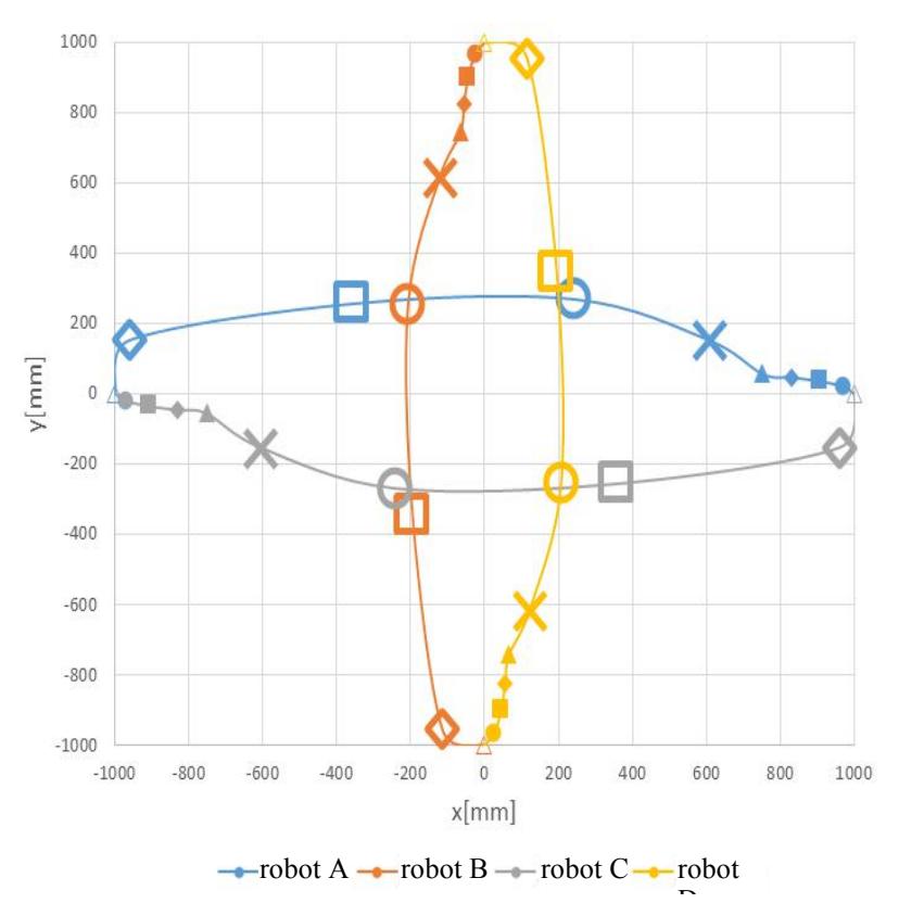
To confirm the performance for collision avoidance, we put four robots evenly spaced apart on the circumference of a circle with the radius of 1000mm. Then, we gave a command to every robot to make moving the opposite point on the circumference as shown in Fig. 14.
Each robot start from the smaller-marker and the coordinates are recorded at a certain interval. The markers(o) show that every robot avoids the collision by moving to the right side. Furthermore, even when the number of robots is increasing as 5 and 6, they also showed the appropriate collision avoidance actions. Consequently, we confirm the avoidance system can perform if the number of robots is increased.
Comparison for the performance of RRT and ORCA in actual robot
We confirmed the actions on the simulation system. So in next, we verified its usability in the actual robots.
Comparison of computational speed
ORCA algorithm is superior in computational speed compared with RRT. To demonstrate this, we measured the time spent to compute the route per one robot. The results are tabulated in Table 1.
Table 1. Comparison of computational speed for RRT and ORCA algorithms
| Average time [ms] | Maximum time [ms] | |
|---|---|---|
| RRT | 7.65 | 18 |
| ORCA | 0.35 | 1 |
It was done under the condition of Windows7 64bit, Core i7-3612QM, 8GB RAM and used chrono (C++ standard library) to measure the time. In RoboCup SSL, instructions to the robots were synchronized with a refresh rate of 17ms. From Table 1, we found that the average time of RRT algorithm was 7.65ms per one robot and resulted 45.9ms in case of 6 robots. Therefore, that calculation might be performed over refresh rate. On the other hand, that of ORCA method was less than 1ms. Thus, the computational speed is suggested about 6ms even at the case of 6 robots. As the results, we confirmed the computational speed by using ORCA algorithm is faster than that of RRT.
Comparison of collision frequency
Although we confirmed the modification for computational speed as described above, if the collision frequency is largely increased, it is no good. Therefore, we evaluated the collision frequency among the 4 real robots of same team. To evaluate it, we use the time of STOPGAME which robot cannot touch the ball but can be arranged. So, we count the frequency of near-miss and actual collision of the robots during the moving. As the results, the probabilities of collision is calculated as tabulated in Table 2. Additionally, we also performed similar experiment under the condition added fixed three markers indicate enemies on the field. The results are tabulated in Table 3. These results of ORCA algorithm looks like better than that of RRT in our limiting condition. In table3, it is shown that RRT algorithm had difficulty making path finding, because of the density of the robots including markers on the field was raised. As the results, the collision might be increased. On the other hands, in case of ORCA algorithm, the collision probability stayed about the same (lower than 30%) in both of Tables 2 and 3. The details of the reason why collision probability of ORCA algorithm is better than that of RRT are unclear. It might be depend on the characteristics of robots and/or experimental condition. Nevertheless the ORCA method was shown to be useful for SSL. The collision for ORCA algorithm might be caused by setting the exact size of robots in AI system. Therefore, it will be lower the collision probability induced by missing control of robots and/or the information error of the camera by use of proper margin taken into account the robot's size on AI.
Table 2. Comparison for collision probabilities of 4 robots on RRT and ORCA
| probability of collision [%] | |
|---|---|
| RRT | 35.00 |
| ORCA | 27.27 |
Table 3. Probabilities for collision in case of 4 allies and 3 enemies put on the field
| probability of collision [%] | |
|---|---|
| RRT | 45.00 |
| ORCA | 21.74 |
Comparison for travel time
It is easy to avoid collision at low speed but such a situation may not occur in actual game. So, we also evaluated the travel time comparing the RRT and ORCA under the same condition as previous section (four ally robots and fixed three enemies). The results are summarized in Table 4.
Table 4 shows that the travel time of ORCA algorithm is about 25% less than that of RRT. This might be referred that ORCA was repeated acceleration and deceleration of the robots depending on the nearby situation, while RRT is always done at the maximum speed. It seems that ORCA algorithm looks like better than RRT in terms of computational speed, and the performance of collision avoidance in practice game at actual field is also good. Although collision is happened, the collision avoidance system is worked so well compared with previous our system. However, the present ORCA system is no good in respect of travel time now. So, we have to improve moving speed of robot while the current probability of collision is maintaining. Up to now, we may not be able to evaluate it sufficiently on our system in various situations, for example, the enemy robots are moving. Therefore, we are going to verify this system in practice games and next coming Japan Open and try to maintain the improvement for collision avoidance and moving speed of robots.
Table 4. Comparison of travel times of 4 robots on RRT and ORCA algorithms
| average travel time [s] | maximum travel time [s] | |
|---|---|---|
| RRT | 10.46 | 21.72 |
| ORCA | 13.21 | 25.89 |
References
- T. Sano, S. Okuda, K. Matsuoka, Y. Yamauchi, H. Yokota, T. Sakaguchi, M. Watanabe, T. Sugiura: KIKS 2015 Team Description Paper, http://www.ee.toyota-ct.ac.jp/~sugi/RoboCup.html
- https://github.com/msgpack-rpc/msgpack-rpc/blob/master/spec.md
- M.Tokic: Adaptive ε-greedy Exploration in Reinforcement Learning Based on Value Differences, http://www.tokic.com/www/tokicm/publikationen/papers/AdaptiveEpsilonGreedyExploration.pdf
- K. Dolan: Genetic Programming Source, http://geneticprogramming.us/Selection.html
- J. Bruce and M. Veloso : Real-Time Randomized Path Planning for Robot Navigation, RoboCup 2002: Robot Soccer World Cup VI, vol. 2752, pp. 288-295 (2003)
- J. van den Berg, S. Guy, M. Lin, D. Manocha: Reciprocal n-body Collision Avoidance Robotics Research, vol. 70, pp. 3-19 (2011)
- T. S. Ferguson: LINEAR PROGRAMMING a Concise Introduction, http://www.math.ucla.edu/~ tom
- J. van den Berg, J. Snape, S. Guy, D. Manocha: Reciprocal Collision Avoidance with Acceleration-Velocity Obstacles, Robotics and Automation (ICRA), 2011 IEEE International Conference on, pp. 3475-3482 (2011)