MCT Susano Logics 2016 Team Description
Shota Aoki, Taihei Degawa, Kazuhiro Fujihara, Yuta Notsu, Toshiyuki Beppu
National Institute of Technology, Matsue College, 14-4, Nishi-Ikuma, Matsue, Shimane, 690-8518, Japan
Abstract In the RoboCup Small Size League (SSL), teams of six robots which are autonomously controlled by a team AI play soccer games using an orange colored golf ball. In SSL games, an image processing system (SSL-Vision) receives images from four cameras which are installed 4 meters above the field surface, identifies the robots and ball positions. Because the SSL-Vision identifies the robots and the ball positions from all camera images, multiple position coordinates are computed in overlapping regions of the images. A multi-particle filter was developed to determine the ball position in the overlapping regions, and to minimize the discontinuity of the moving ball locus across the regions. The multi-particle filter consists of 4 particle filters and a particle binder estimates the position of the ball from the median point of a combined distribution. In an experimental setup, the multi-particle filter smoothly connected two ball locus vectors with a distance of 17 mm. The distances between each sample of the filtered outputs were almost the same as both sets of data from the two cameras.
Keywords. Particle Filter, SSL-Vision.
1 Introduction
From RoboCup 2014 João Pessoa, Brazil, a "large field" of nominal size 9000 mm * 6000 mm was partially adopted for SSL games. At RoboCup 2015 Hefei, China, all SSL games were played on the large field.
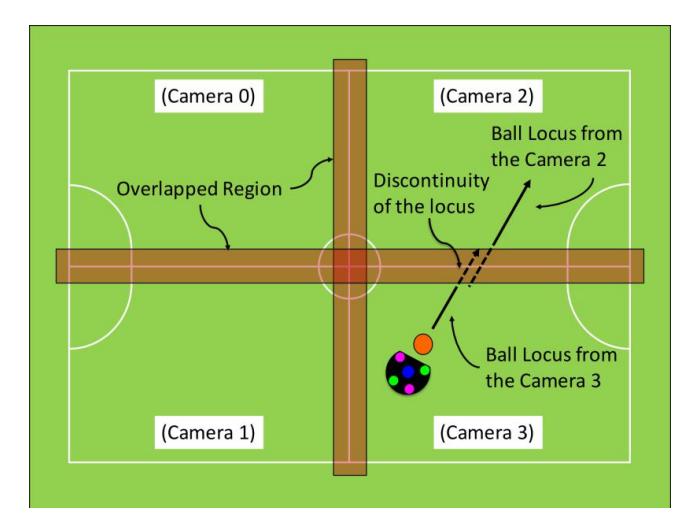
In SSL games, an image processing system (SSL-Vision) [1] identifies the robots and the ball positions at a speed of 60 frames per second from images taken by four cameras installed at 4 meters above the field surface. The SSL-Vision calculates the coordinates of the robots and the ball, and sends position data to the team's AI computers. Because the SSL-Vision identifies the robots and the ball from all camera images, multiple position coordinates are computed in overlapping regions at boundaries between camera images (Fig. 1).
At the game kickoff, a ball was placed on the center of the field, where four cameras capture images and the SSL-Vision outputs four coordinates of the ball simultaneously. Our team AI vacillated between position data and therefore, could not control the kicker robot accurately. Furthermore, the overlapping region across the goal caused fluctuations in our AI's predicted ball locus and resulted in the poor defense of our goalkeeper. A multi-particle filter for the ball position estimation was developed to determine the coordinates of the ball in the overlapping regions, and to minimize the discontinuity of the moving ball locus across the boundaries.
2 Multi-Particle Filter
2.1 Particle Filter
A Particle Filter (PF) is a set of genetic-type particle Monte Carlo methodologies to solve the filtering problem [2]. Each particle in the PF has the state vector. The PF estimates the posterior density of the state vectors from given observation vectors.
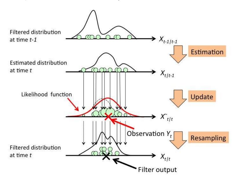
Figure 2 shows the process of the PF [3]. The PF consists of three calculation steps of estimation, update and resampling. At the start of the loop of the process, the PF generates a set of particles based on the uniform distribution or the normal distribution. From the second loop, the PF uses the anterior filtered distribution of the system to estimate the current state. The samples from the distribution are represented by a set of particles.
The PF estimates a state distribution at time $t$ ($x_{t|t-1}$) from that of $t - 1$ ($x_{t-1|t-1}$), utilizing the system model in the estimation step. In the update step, the PF receives an observation vector $y_t$ and sets a probability density function. Then the PF evaluates a probable weight of each particle that represents the probability of that particle being sampled from the function ($x_{t|t}$). In the resampling step, the PF adjusts the distribution to the observation by weighted random sampling of the particles with the probable weights from the estimated distribution at time $t$. After the resampling step, the particle distribution ($x_{t|t}$) shows the filtered distribution at time $t$. The PF outputs the median point of the filtered distribution $\hat{x}$ as the estimated state of the system.
2.2 Particle Filter for SSL-Vision
A two-dimensional state vector $x_t$ indicates the coordinates of the ball position [$P_{xt}$, $P_{yt}$].
$$\boldsymbol{x}t = \begin{bmatrix} p{xt}, & p_{yt} \end{bmatrix} \tag{1}$$
An observation vector $y_t$ is the coordinates of the ball position received from the SSL-Vision. Observation noise $w$ is the normal distribution with a standard deviation of 2 millimeters. This value was decided experimentally.
$$y_t = x_t + w$$
$$w \sim N(\mathbf{0}, \mathbf{R})$$
$$\mathbf{R} = diag(4.0, 4.0)$$
A velocity vector $s_t$ is calculated from the PF output of $\hat{x}t$ and $\hat{x}{t-1}$, and the sampling period of the SSL-Vision $\Delta t$.
$$\mathbf{s}_t = \left(\widehat{\mathbf{x}}t - \widehat{\mathbf{x}}{t-1}\right) / \Delta t \tag{3}$$
A system model is defined as follows.
$$x_t = x_{t-1} + s_{t-1} * \Delta t + v$$
$$v \sim N(\mathbf{0}, \mathbf{Q})$$
$$\mathbf{Q} = diag(1.0, 1.0)$$
An inaccuracy of the ball motion is expressed as system noise $v$. This system noise conforms to the normal distribution with a standard deviation of 0.5 millimeter.
The probable weights of the particles are calculated from a normal distribution with the state vector $x_t$ and the observation vector $y_t$.
$$\omega_t = \frac{1}{\sqrt{2\pi R}} exp\left(-\frac{(x_t - y_t)^T R^{-1}(x_t - y_t)}{2}\right) \tag{5}$$
2.3 Multi-Particle Filter
The SSL-Vision identifies the robots and the ball position from all camera images and therefore, multiple position coordinates are computed in the overlapping regions of the images. A multi-particle filter (MPF) was developed to determine the ball position in the overlapping regions, and to reduce the data discontinuity of the moving ball, which goes across the boundary between camera areas.
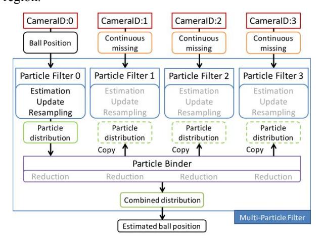
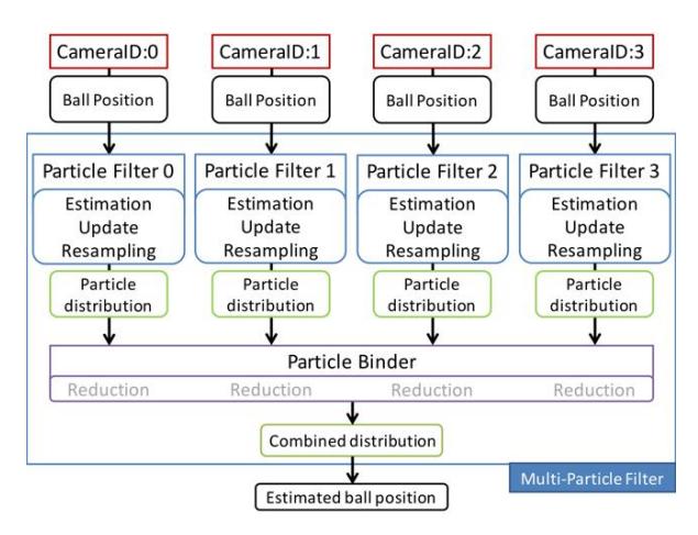
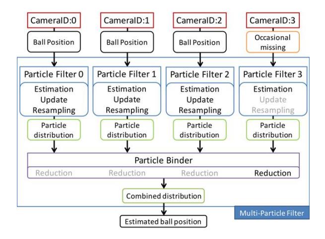
Figure 3 shows the process of the MPF. The MPF consists of four PFs and a particle binder. Each PF is assigned to a designated camera. The SSL-Vision sends the ball position data with camera IDs. The MPF identifies the data from the ID number and each PF calculates a particle distribution for the camera independently. The particle binder combines the filtered distributions and outputs the median point of the combined distribution $\hat{x}$ as the estimated ball position.
When the ball is in a camera area, a PF for the received data executes the filtering process (estimation, update and resampling) as shown in Fig. 3. The PFs with continuously missing data will not execute the filtering steps. The particle binder copies the particle distribution from the executed PF to the combined distribution and calculates the median point. Then the particle binder sends the distribution to other PFs of continuously missing data as the anterior distribution for the next filtering. This technique reduces fluctuations of the estimated ball position for the time of the ball entry to the overlapping region.
2.4 Experimental Result of the MPF
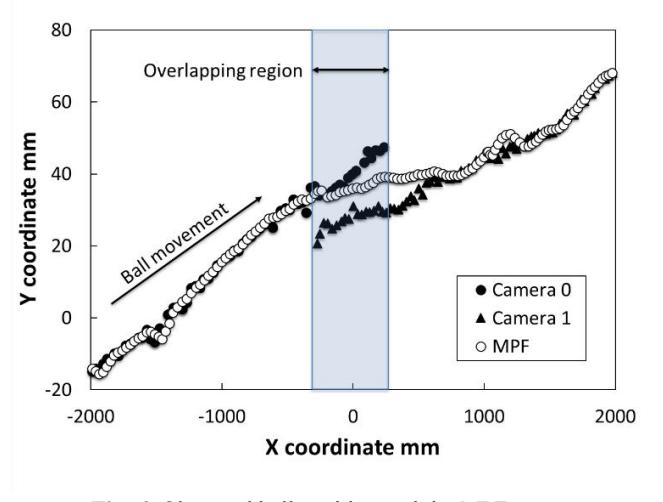
Two cameras (AVT Stingray F046C, 780 x 580 pixels) at a distance of 3 meters installed 3.4 meters above the surface of the field monitored a field of 6 by 4.5 meters with an overlapping region of 620 millimeters in width. A ball, which went across the overlapping region at a speed of 1.9 meters per second was captured by cameras. The MPF outputs were calculated offline. The number of total particles, pMAX, was set to 300, and the maximum calculating cycles of data missing, missingMAX, was set to 15.
Figure 6 shows the camera captured coordinates and the estimated position of the MPF. The distance of the ball locus vectors of camera 1 and 2 is about 17 millimeters. The MPF estimation connects the locus smoothly. The distances between each sample were 32 ± 15 (Camera 0), 28 ± 9 (Camera 1), and 28 ± 6 (MPF) millimeters in this trial.
3 Implementation of MPF to the Team AI
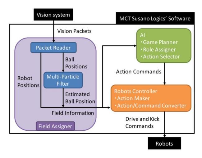
Figure 7 shows the software structure of MCT Susano Logics. Packet Reader receives vision packets from the SSL-Vision and sends the ball position with camera ID to the MPF. The estimated position is sent to both AI and Robots Controller. The software was developed by C++ (GCC 4.9). The process time of the MPF with 250 particles is 2.41 ± 0.37 milliseconds on Dell Inspiron 15 5000 (CPU: Intel Core i7-5500U 2.4GHz, memory size: 8GB) with Linux OS (Xubuntu 14.04). The speed of the MPF is adequate for our needs and we will implement it into our team AI.
References
- S. Zickler, T. Laue, O. Birbach, M. Wongphati, M. Veloso. SSL-Vision: The Shared Vision System for the RoboCup Small Size League. 2009. http://isites.harvard.edu/fs/docs/icb.topic859418.files/papers/sslvision2009-new.pdf
- P. Del Moral. Non Linear Filtering: Interacting Particle Solution. Markov Processes and Related Fields 2 (4): 555–580, 1996.
- T. Ikoma. Sequential Monte Carlo method and Particle Filter (in Japanese). Chapter 11, Statistical Science in 21th. Century, Japan Statistical Society. 2008. http://ebsa.ism.ac.jp/ebooks/sites/default/files/ebook/1881/pdf/vol3_ch11.pdf