MRL Extended Team Description 2016
Amin Ganjali Poudeh, Mohammad Sobhani, Adel HosseiniKia, Alireza Karimpour, Sina Mosayeb, Hamed Mahmudi, Saeid Esmaeelpourfard, Meisam Kassaeian Naeini, Aras Adhami-Mirhosseini
Islamic Azad University of Qazvin, Electrical Engineering and Computer Science Department, Mechatronics Research Lab, Qazvin, Iran
Abstract MRL Small Size Soccer team, with more than seven years of experience, is planning to participate in 2016 world games. In this paper, we present an overview of MRL small size hardware and software design. Having attained the second place in 2015 and third place in 2010, 2011 and 2013 competitions, this year we enhanced reliability and achieved higher accuracy. Due to enlargement of the field, we had to change some parts of software code from low level control to high level strategies. Finally, by overcoming electronic and mechanical structure problems, we promoted the robots ability in performing more complicated tasks.
1 Introduction
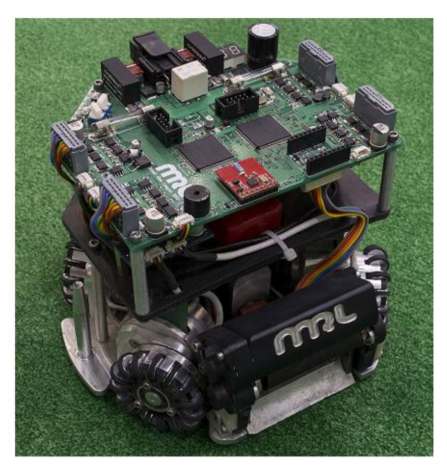
MRL team started working on small size robots from 2008. In 2015 Robocup, the team was qualified to be in semi-final round and achieved the second place. In the last competition in China MRL team ranked in the top 3 teams. In the upcoming competitions, the team goals are, first: preparation for double-sized field games and, second: having more dynamic and intelligent behavior. In 2016 competitions the main structure of the robots is the same as last year, see [1] for details. Figure 1 shows the MRL 2016 robots.
Some requirements to reach this target are achieved by redesigning the electrical and mechanical mechanisms. Moreover, simple learning and optimization approaches are employed in the way of more dynamic play. Evaluation by software tools, like online debugger and simulator which is detailed more in [2], made the design procedure and verification faster.
This paper is organized as follows: First of all, the software architecture which includes our approaches in high level strategies, defense algorithms with details are described in section 2. The Electrical design including ARM micro controller together with FPGA, and other accessories of robots onboard brain, is explained in section 3. Description of new mechanical structure, which modifies the capabilities of the robots dribbler system, is the subject of section 4.
2 Software
In this part the software main objects are presented. It is shown that how our new modifications provide us a more intelligent and flexible game. In this year
MRL software team has not changed the AI main structure. The game planner as the core unit for dynamic play and strategy manager layer is not changed structurally, but some new skills and abilities are added to the whole system. In this section, after a brief review about the AI structure, short description of the unchanged parts are presented and references to the previous team descriptions are provided. Finally major changes and skills are introduced in details.
The software system consists of two modules, AI and Visualizer. The AI module has three sub-modules being executed parallel with each other: Planner, STP Software (see [7]) and Strategy Manager. The planner is responsible for sending all the required information to each section. The visualizer module has to visualize each of these sub-modules and the corresponding inputs and outputs. The visualizer also provides an interface for online debugging of the hardware. Considering the engine manager as an independent module, the merger and tracker system merges the vision data and tracks the objects and estimates the world model by Kalman Filtering of the system delay. Figure ?? displays the relations between different parts. In this diagram, an instance of a play with its hierarchy to manage other required modules is depicted. The system simulator is placed between inputs and outputs and simulates the entire environment's behavior and features. It also gets the simulated data of SSL Vision as an input and proceeds with the simulation.
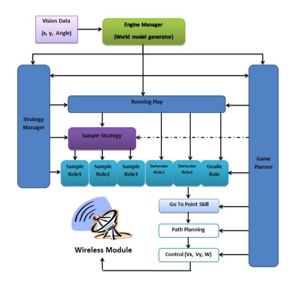
Many parts of AI system are the same as before that are described in the last years ETDPs. The following list describes these parts breifly, while the references for details are mentioned for each part.
– Some techniques and skills like space dribble and chip dribble are introduced in [5].
- Visualizer and online debugging system as useful tools for fast improvements are discussed in [5] and [3].
- Game planner and some main features of it (e.g. regioning) are described in [4].
- Role assigner as an important part of STP structure is mentioned in [3].
- Defense analyzer as an auxiliary tool to understand the defense strategy of the opponent are introduced in [2].
- Motion planner and navigation system consists of the RRT path planner and trajectory generation method are discussed in [3]. A heuristic method that uses the maximum robot ability of motion on the generated path is introduced there.
- Model predictive control for trajectory tracking is introduced in [2] for small size robots. Details and results of the suggested methods can be found in [6].
In the following subsections we introduce improvements and modifications in details. Note that, the arrangement of the introduced approaches is to increase tractability.
2.1 Strategy management
Last year we introduced a new layer of MRL AI hierarchy, the Strategy Layer. In the strategy layer, the AI system learns to select the best game strategy for some specific time frames. Each strategy is a heuristic game playing for certain number of attendees. "Field region game status" and minimum score to be activated" are parameters pertaining to each strategy. For instance, Sweep and Kick strategy with three attendees that works well in the middle of the field is activated after score one, and requires Indirect Free Kick" game status. If all four parameters are satisfied, the strategy becomes "applicable" at certain time frame. We model each strategy as a Finite State Machine (FSM). Consecutive states of strategy FSM indicate the chain of actions required to be performed in that strategy. The transition conditions between states reflect the prerequisite conditions for the actions. The FSM has an initial state with which the "applicability" is verified. It also has got Trap and Finish states indicating "failed" and "successful" ending of the strategy, respectively. A dynamic score is designed for each strategy. After completion of each strategy (either failed or successful), the strategy score is updated. Also the strategy score will be updated based on the result of the game analysis achieved from the game planner and opponent defense analyzer during the game.
Strategy manager operates as the highest component of the Strategy Layer. This component is responsible for selecting the best strategy at each time frame. The strategy manager has three different selection policies:
- Random Selection: The manager randomly selects one of the applicable strategies.
- Higher Score with a Probability of Random Selection: The manager tends to select the strategy with the highest score as of now, trying to apply
the best strategy which has proved to have the best performance. Also, for the sake of giving the chance to some lower scored strategies to make progress, the manager randomly selects a strategy with probability of P.
- Weighted Random Selection: The manager randomly selects one of the strategies, each of which has a weight corresponding to the probability to be selected.
The Strategy Manager selects one of the applicable strategies in one of the three mentioned ways and the roles for performing the strategy are assigned to the attendee robots. When the strategy traps or successfully ends, roles for the normal play are reassigned to the robots. The strategy layer helps us to avoid a share data or blackboard for agents. Therefore we can design a cooperative game of agents, dynamically.
2.2 Prioritizing opponents robots
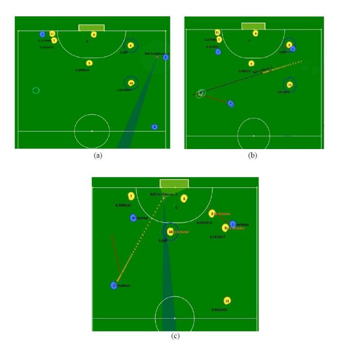
This part plays the main role in defensive tactics. It is very important to cover opponent attack strategy with a reliable defense. In defensive tactics, due to the robots high speed and accuracy, each mistake can lead to a goal chance for the opponent. On the other hand, owing to the various attacking strategies used by different teams, covering all possible game conditions needs a lot of parameters and that raises the chance of mistakes. Collecting all these parameters and finding proper relation between them is a very hard or even impossible task. We calculate a score between 0 and 1 for each opponent robot in each frame. This score shows opponent robots importance. This score must be very reliable in all opponent attack conditions. In order to reduce the complexity we have divided this operation to two parts offline sampling and online calculation.
Offline Sampling
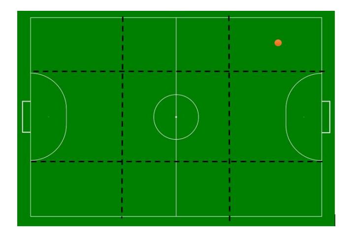
In this part the field is divided to 9 regions as into Figure 3. By putting the ball in the center of each region, to increase scores reliability, a set of scores obtained by human perception will be assigned to 24 critical points of the field. Consider pb(i) = (xb(i), yb(i)) i = 1, .., 9 center of each region. For each of these positions define pr(j) = (xr(j), yr(j)) j = 1, .., 24 positions for points to be scored. s(i, j) shows the importance (score) of position j when the ball is in position i.
Online Calculations
To compute the score for each opponent robot, there are two situations in the game:
An opponent robot owns the ball: Suppose the ball owner is in position (x0, y0). For an opponent robot in position (xs, ys) we compute the importance score as score(xs, ys). First of all we define ϕ(i, j) and ϕt(i, j) as:
$$\varphi(i,j) = \exp\left(-\frac{(x_s - x_r(i,j))^2}{\sigma_x^2} - \frac{(y_s - y_r(i,j))^2}{\sigma_y^2}\right)$$ (1)
where $\varphi(i,j)$ shows how much the opponent robot belongs to the predefined position $p_r(i,j)$ . $\sigma_x^2$ and $\sigma_y^2$ are variances of Gaussian function that are used to adjust the validity of each point domain.
$$\varphi_t(i) = \exp\left(-\frac{(x_0 - x_b(i))^2}{\sigma_{xt}^2} - \frac{(y_0 - y_b(i))^2}{\sigma_{yt}^2}\right)$$ (2)
where $\varphi_t(i)$ shows how much the ball owner belongs to the predefined ball position $p_b(i)$ . $\sigma_{xt}^2$ and $\sigma_{yt}^2$ are variances of Gaussian function that are used to adjust the validity of each point domain.
Now, $s_t(i)$ is defined as the predicted normalized score of opponent robot at at $(x_s, y_s)$ with speed of $(v_x, v_y)$ if the opponent ball owner is exactly in the predefined ball position $p_b(i)$
$$s_t(i) = \bar{s}(i) + \left(\frac{\partial \bar{s}(i)}{\partial x_s} v_x + \frac{\partial \bar{s}(i)}{\partial y_s} v_y\right) \Delta t \tag{3}$$
where $\bar{s}(i)$ is the normalized score of the static opponent robot if the ball owner is exactly in the predefined ball position $p_b(i)$ .
$$\bar{s}(i) = \frac{\sum_{j=1}^{24} s(i,j)\varphi(i,j)}{\sum_{j=1}^{24} \varphi(i,j)}$$ (4)
Parameter $\Delta t$ used is as prediction horizon of scoring for a moving opponent robot, Figure 4. Finally, the opponent score for an arbitrary position of the ball owner is computed as:
$$score(x_s, y_s) = \frac{\sum_{i=1}^{9} s_t(i)\varphi_t(i)}{\sum_{i=1}^{9} \varphi_t(i)}$$ (5)
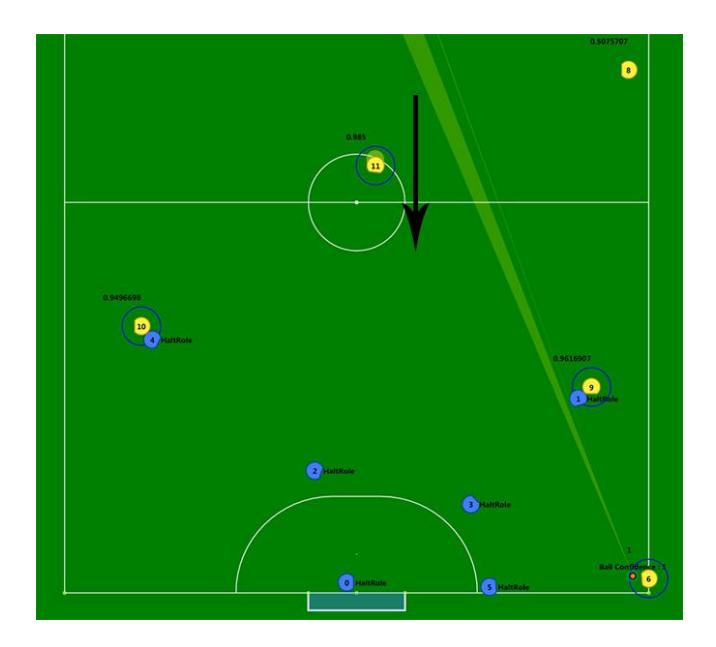
No opponent ball owner exists: In this situation depend on the ball position and velocity and opponent robots' positions with a heuristic function we guess the next opponent ball owner. After selecting the future ball owner the same calculations leads to the each robot importance score.
2.3 PassShoot strategy
Simple pass and shoot is one of the most common strategies in SSL owing to its high execution speed. On the other hand due to the improvement of SSL teams in marking and defense tactics, it is very hard to achieve success with simple pass and shoot strategy with two attended robots. The proposed pass and shoot strategy has been implemented with three robots, a passer and two positioners, Figure ??. Moreover, to increase the chance of success, the strategy has been implemented in the most possible dynamic way. In this strategy one of the positioners is selected to get the pass. The selection is made at the last moment of the passing state of the strategy. It depends on the situations (position, clearance) of two positioners. Due to this type of selection, it is not clear which robot kicks the ball. In order to make the strategy dynamic, we use a synchronizer module. This module synchronizes passer with the positioners in the way that pass point is reached by the ball and the selected positioner simultaneously. The synchronization method considers the conflicts and obstacles. This module calculates the wasted time and then makes up this time by changing operations time-line. Thanks to the synchronizer, it is not necessary for the shooter robot to be in the pass point from the beginning. This increases the chance of success. The pass point is determined by the game planner module using a grid based algorithm according to some parameters like goal view angle, opponents density in different regions of the field. Type of pass (direct or chip) depends on the obstacles in the way of pass point. It can be changed until the time of kicking.
Synchronization algorithm This module is used for synchronizing between passer and shooter robots while unexpected causes such as obstacles in the way of shooter robot does not make any disturbance in the pass-shoot time-line. To this end parameter tm is defined as the time it takes the shooter robot to reach the pass target in an obstacle free path and tp is defined as the time it takes the ball to reach the pass target from beginning of the pass procedure. tp and tm are determined as below:
tm = km · motionT ime ps(0), pt
tp = kp ·
      passT ime (passSpeed, pt) + motionT ime
                                                  pp(0), pb
                                                          + two
where
two: An offset waiting time
ps(i) : Shooter robot position at frame i of the procedure
pp(i) : Passer robot position at frame i from the beginning of the procedure
pb: Ball first position
pt: Pass target position
km and kp: Constants
motionT ime is an experimental/heuristic function that estimates the time it takes a robot to reach a target from an initial point.
passT ime function calculates the time it takes a passed ball to reach a target with an initial pass speed considering both rolling and slipping parts of the ball motion.
Considering these definitions the pseudo code of synchronization function is as below:
isInP assState = goP ass(passT arget, tw); if isInP assState then counter + +; if tp > tm then if counter ≥ tp − tm then goT oP oint(shooterRoboto, passT arget); determineW aitingT ime = true; else determineW aitingT ime = f alse; stop(shooterRobot); end else gotoP oint(shooterRobot, passT arget); determineW aitingT ime = true; if counter < tm − tp then two + +; end end else counter = 0; stop(shooterRobot); end tw = two; if determineW aitingT ime then twe = calculateExtendedW aitingT ime(); tw = tw + twe; end
goP ass function generates proper commands for robot to go behind the ball and throw a pass to an specific passT arget after waiting for tw frames. It returns a Boolean flag which indicates if there is any obstacle between passer robot and the ball.
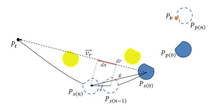
calculateExtendedWaitingTime function determines extended waiting time depends on the deviation of the shooter robot from the straight (obstacle free) path. For this purpose $v_r$ is defined as the reference coordinate as below:
$$\boldsymbol{v_r} = p_t - p_s\left(0\right)$$
We use a near-time optimal trajectory planner implemented as the function of
$\langle V_{ideal}^, X^ \rangle = motion 1 Din Refrence \left( P_{s(0)}, p_t, r \right)$ to compute the sequence of velocity commands $V_{ideal}^$ and the position $X^$ required to navigate from initial location $p_{s(0)}$ to $p_t$ along $v_r$ with final velocity of zero, see Figure 6. To compare the motion of the shooter robot with an ideal motion along $v_r$ , $d_x$ and $d_r$ are determined as below:
$$d = P_s(n) - p_s(n-1)$$
$$R = P_s(n) - p_s(0)$$
$$dr = |R| \cdot Cos(\widehat{R, v_r})$$
$$dx = |d| \cdot Cos(\widehat{d, v_r})$$
where
d: Displacement vector of shooter robot in the last frame
R: Displacement vector of shooter robot from the initial point
dx : Projection of $\boldsymbol{d}$ on $\boldsymbol{v_r}$
dr: Projection of $\boldsymbol{R}$ on $\boldsymbol{v_r}$
Finally, the extended waiting time $t_{we}$ is calculated from the following equations.
$$v_d = V_{ideal}^* (dr)$$
$$t_{w_e} = \int_{t_n}^{t_0} 1 - \frac{d_x}{v_d}$$
where:
$v_d$ : Desired velocity at distance of dr from $p_{s(0)}$ along $v_r$
$t_{we}$ : Extended waiting time of the passer
2.4 Simple Motion Planning
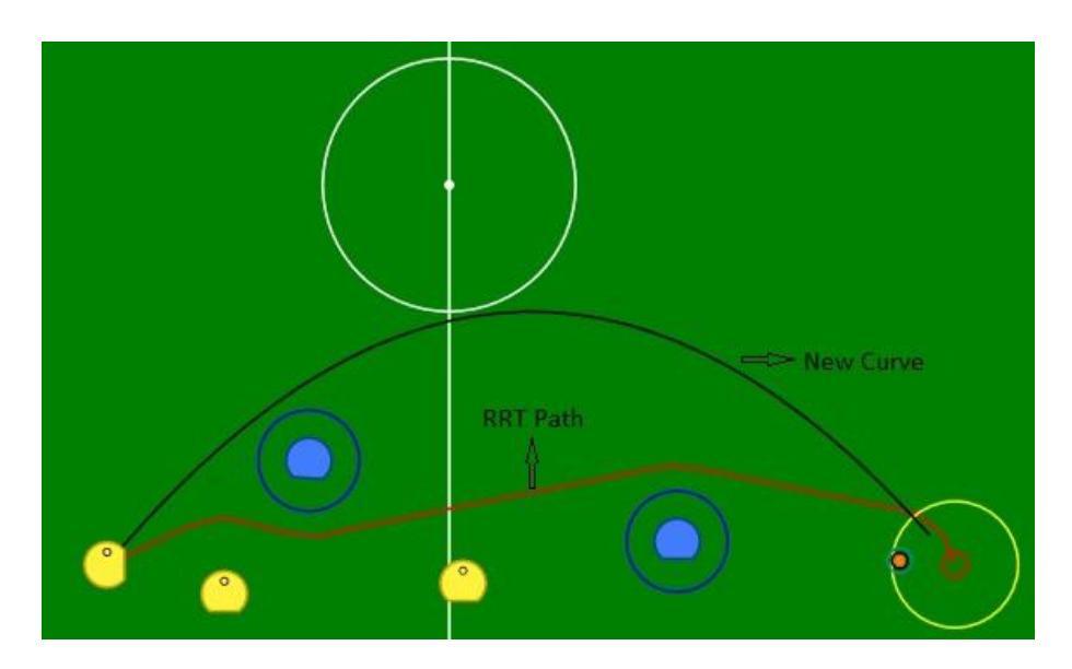
Our motion planner has been changed to the sake of complexity and heavy processing of Rapid Random Tree (RRT) and with respect to the new size of the field, the new planner is combination of preprocessed and simple paths like a curve.
At the beginning number of simple paths has been generated in order to a robot and the target which is consisting of a straight line, simple polynomial curves and also sinus curves. Next each path is being checked by all obstacles in field and in the next stage an optimization finds the best path with respect to our parameters and cost function. Velocity and instantaneous acceleration has been calculated by result of first and second derivation of path equation and finally they return as control parameter to low- level control unit.
For instance:
$$Y = x^2$$
Speed Constraints are being considered as bellow:
$$V_x^2 + V_y^2 \leqslant V_{max}^2$$
$$V_Y = 2x \cdot V_x$$
$$(2 \cdot x \cdot V_x)^2 + V_x^2 \leqslant V_{max}^2$$
$$4x^2 \cdot V_x^2 + V_x^2 \leqslant V_{max}^2$$
$$V_x = (V_{max}^2 \setminus 4x^2 + 1)^{\frac{1}{2}}$$
Also acceleration Constraints are being considered as bellow:
$$a_x^2 + a_y^2 \leqslant a_{max}^2$$
$$a_y = 2V_x^2 + 2x \cdot a_x$$
$$(2V_x^2 + 2x \cdot a_x)^2 + a_x^2 \leqslant a_{max}^2$$
$$(4x^2 + 1) \cdot a_x^2 + (8x \cdot V_x^2) \cdot a_x + 4V_x^4 \leqslant a_{max}^2$$
where:
Vx: Linear Velocity of x
Vy: Linear Velocity of y
ax: Linear Acceleration of x
ay: Linear Acceleration of y
amax: Maximum Linear Acceleartion of Robot
x: Position of x
y: Position of y
Our new motion planner decreases the complexity of processes because it does not have any intermediate points like RRT additionally the improvement increased the speed of robots to move through the pass.
2.5 Shamsae Skill
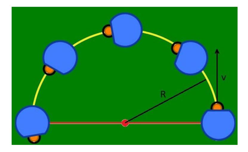
The aim this skill is catching the ball inversely and move the ball through the half-circle path with respect to the rules(1 meter displacement of ball). This movement is totally open loop without any feedback from vision. Direction and radius of half-circle have been chose Due to the obstacles. (Linear Acceleration) always considered maximum value:
$$V = (a \cdot R)^{\frac{1}{2}}$$
$$\omega = (V \setminus R) \cdot K$$
where:
K: Cte
V : Linear Velocity ω: Angular Velocity a: Linear Acceleration
R: Radious x: Position of x
K is a coefficient which has been set manually and it is releatedto the distance of ball from spin back .
2.6 Defenders positioning algorithm
In Small Size League matches (like real soccer games) attacking strategies are very flexible and dynamic. This feature, implies that the defense strategies should be dynamic too. In fact, there are lots of unforeseen states that cannot be considered in advanced. Thus, defenders cannot classify all of them to have suitable react. Between the defense skills, positioning is the most important one. Positioning is the sequence of finding the target(s), selecting the blocking strategy. In the last years, we used a fixed form of defense (i.e. two defenders with goal-keeper between them). This year we are going to test the new positioning strategy. This strategy is based on an optimization. We prefer to perform it online. Defining a good set of cost function and constraints is the first step in optimization. The cost function, calculate the cost of each react of our defenders. We consider that our problem could solve better in multi-objective optimization so we implemented two different main cost functions.
Using meta-heuristic and gradient-base optimization algorithms helped us to solve these problems.
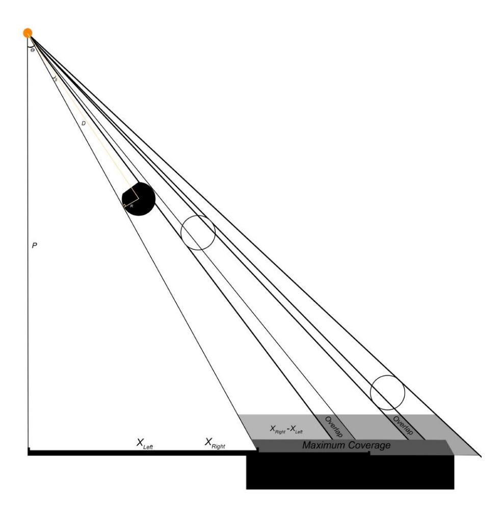
First Cost Function has focus on maximum coverage of the goal line. Followings, we calculate empty points of the goal based on the Figure 9.
$$x_{left} = p \tan \left(\Theta - \sin^{-1}\left(\frac{R}{D}\right)\right) x_{right} = p \tan \left(\Theta + \sin^{-1}\left(\frac{R}{D}\right)\right)$$ (6)
After calculation of all 6 Points on the goal Line, we exclude the overlaps. So we have strict value of goal coverage.
$$GoalCoverage = (X1_{Right} - X1_{left}) + (X2_{Right} - X2_{left}) + (X3_{Right} - X3_{left}) - OverlapValue$$ (7)
Finally optimization algorithm tries to find minimum of GoalEmptyValue =1- GoalCoverage. Other objective functions that are considered with the GoalEmptyValue are defenders' distance from the qoal line and from the their last positions.This set of objective functions, results in th maximum coverage of goal with possible minimum displacement and minimum distance to goal center.
Another cost function calculates the perpendicular distance of each robot to virtual line from ball to some goal points line that helps us to consider the time dimension. This optimization has some constraints according to the rules of SSL 2015 all robots except Goal-Keeper cannot go to the penalty area and some other constraints that consider in our optimization. To find the best solution Particle Swarm Optimization (PSO) and Genetic Algorithm (GA) had implemented but PSO has been chosen because it is faster than GA to find the answer in this particular problem. PSO makes use of a velocity vector to update the current position of each particle in the swarm. The position of each particle is updated based on the social behavior that a population of individuals, the swarm in the case of PSO, adapts to its environment by returning to promising regions that were previously discovered. The process is stochastic in nature and makes use of the memory of each particle, as well as the knowledge gained by the swarm as whole, [11]. After implementation, we set the optimization parameters as 1000 Iterations and 10 particles. Without any parallelism it gives the suitable answer in less than 300 Microseconds that is still too much. We are trying to reduce the process time by using GPU programming and adding some more constraints to make the search space smaller.
2.7 Penalty Goal Keeper
In small size league, penalties are converted to goals more often than not. Missed penalty kicks are often caused by the kicker robot not the reaction of the keeper. This is mainly because of the command delay, ball speed after the kick and short distance of the penalty point to the goal line. This means that if the keeper waits for the kick to find the diving direction, it usually does not reach the ball. The only possible way, is to start the motion several frames before the kick time or force the kicker robot to select the direction that is suitable for keeper. This year we introduce a learning algorithm that tries to guess the penalty shooter's behavior. The method especially focuses on the penalty shootout to determine which team is victorious after a drawn match. In this case, each team at least kicks 5 penalties. The learning algorithm for the goal keeper is a combination of classification and pattern recognition methods. Based on the prior penalty kicks by different teams, we extract and classify different types of penalty kickers' behavior. In particular, 18 main patterns are generated by the main state machine, Figure 10. Some of these patterns describe a simple strategy for kicking a penalty, some others show more complicated behavior that are a combination of simple ones. Each pattern may contains some parameters that tunes the behavior. For each pattern, we find the best reaction of the goal keeper like diving and special movements.
After defining the patterns, we try to find the best pattern that fits the particular penalty kicker. This classification procedure starts by the first penalty kick at each game and resets at the end of the game. Many data are extracted from each penalty kick and converted to knowledge about the kicking pattern. This knowledge, for instance initial angle of kicker robot, last angle of kicker robot and distance to ball before kick, help us to classify the penalty kicks correctly. At each penalty kick, goal keeper has two kind of behavior: saving or exciting. Saving is the reaction that aim to catch the ball, while exciting is the action (or reaction) that tries to reveal an important specification of the kicker behavior. Simple analysis shows that if the kicker robot acts similar to one the
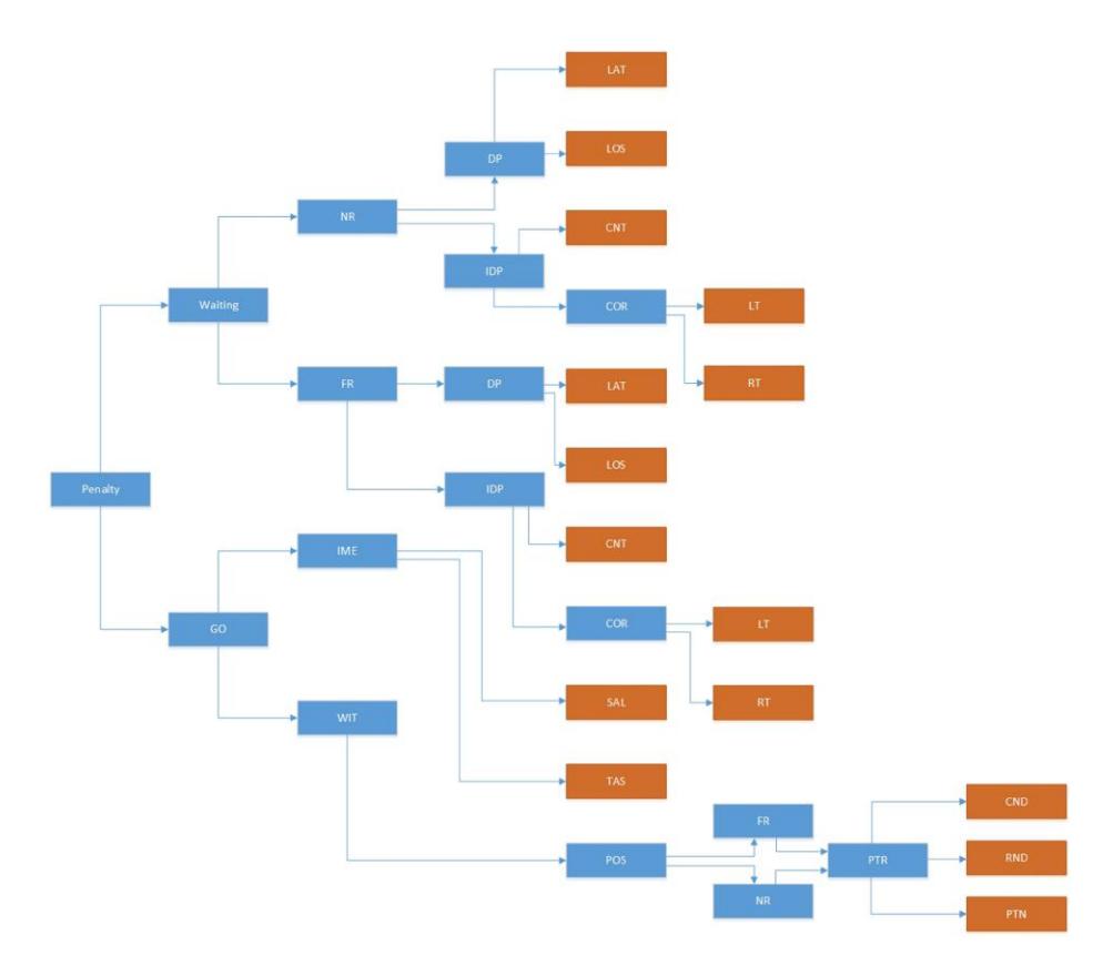
patterns and does not change its behavior, after the third goal keeper will do saving reaction with increasing chance of success.
3 Electronics
MRL robot electronic consists of an Altera Cyclone FPGA linked to an ARM core the same as previous years. Changes during last year in this section is implementation of parallel motor controllers in FPGA, since calculation of PID controllers in software requires a lot of CPU time. Moreover, moving controllers to FPGA, the ARM processor can be dedicated to other tasks with less interrupts. The other changes are using frequency IR sensor for ball detection and some modifications on the wireless board. For unchanged parts of the electronics see [3] and [2].
3.1 Main Board
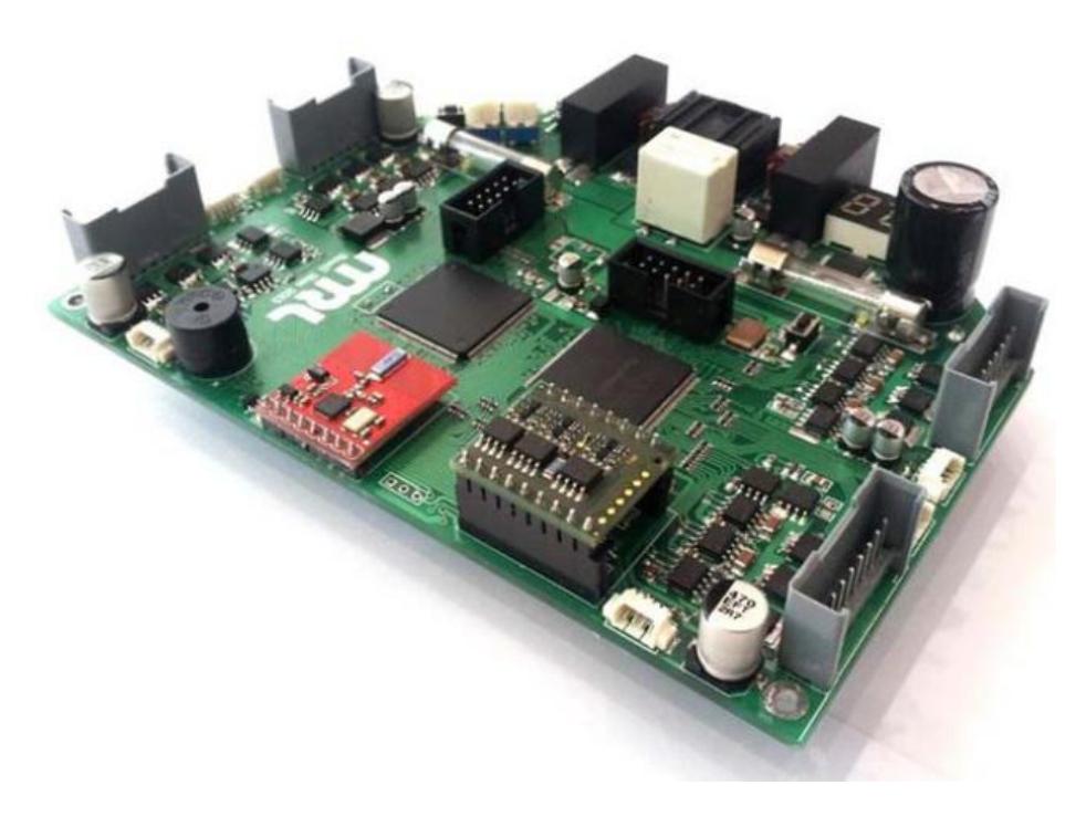
Main board of the robot, which mainly drives wheels and dribbler motors, is illustrated in Figure 11. The board is the same as MRL 2013, [3].
Principle of bootstrap gate driver Signals created from FPGA should turn on the power MOSFETs, but the voltage level of the FPGA pins is not adequate. As a result, MOSFET driver should be used to amplify these signals.
The previous MOSFET driver has voltage supply limitations. Also these drivers can be implemented in the case that the maximum input voltage level is less than the gate-to-source breakdown voltage. While the input voltage level prohibits the use of these drivers, principle of bootstrap gate driver can be taken into consideration. Also previous signals were divided into two parts, logic and power. To transfer the signals between these parts, optocouplers are used. Due to photo-transistor structure of this device, the temperature which rises up in other parts, affects the output voltage level of this device. On the other hand the total delay between transitions is high. Therefore it is essential to replace this part of circuit. Direct driver with ground considering, improves the reliability and increases the switching frequency. For more details see [2].
MOSFET selection Considering the fact that the most of the power loss is related to the RDSon,to reduce power loss we should first choose a RDSon but as a result Qg of the MOSFET is increased. Qg factor defines the time transition in switching and reduces the losses in the gate drive circuit owing to the fact that less energy is required to turn on or off. In optimal design the trade-off between these two factors is important. Since the motor driver frequency is low, RDSon is more important than Qgin in our design. According to the following table which is owned by NXP TM cooperation the PSMN0R9 high performance N-channel MOSFET is selected. Figure 12 lists different MOSFET specifications.
Fig. 12. List of MOSFET specifications.
| Type | Voltage (V) | V os = 4.5 V (mΩ) | V GS = 4.5 V (nC) |
|---|---|---|---|
| PSMN0R9-25YLC | 25 | 0.95 | 51 |
| PSMN1R1-25YLC | 25 | 1.2 | 39 |
| PSMN1R2-25YLC | 25 | 1.35 | 31 |
| PSMN1R7-25YLC | 25 | 2 | 28 |
| PSMN7R5-25YLC | 25 | 8.4 | 7 |
| PSMN9R0-25YLC | 25 | 10.5 | 5.6 |
| PSMN010-25YLC | 25 | 11.9 | 5 |
| PSMN012-25YLC | 25 | 14.1 | 3.8 |
3.2 Low level Controller
The electronic part consists of FPGA and ARM7 microcontroller. Signal processing is managed in FPGA and other tasks like wireless communication, algebraic operation and control task are done in ARM7 core. Among these tasks, the control loop is the most important one.
This architecture faces some problems as:
- Time limitation in perform of control loop due to the high computational cost.
- Suppressing the control loop interrupts by some interrupt event with higher priority.
According to the drawbacks mentioned above, redesigning this structure seems essential. Implementation of PID control loop in FPGA, eliminates these constraints with lowest software and hardware cost. There are two ways to solve the problems:
- Utilizing a soft core like Nios embedded-processor for Altera FPGA.
- Self design architecture and implementation for PID in FPGA.
The first way causes over hardware designing. It is not an optimal way, since the ARM architecture is more powerful than other soft cores. Thus, to design and implement PID control loop in FPGA, we select the second way based on [8].
3.3 Ball detector
To recognize the ball position in dribbler we used and inferred sender and transmitter and reading them with ADC unit in ARM. As it is mentioned in the last year ETDP, we use IR sender sensors currently with specific frequency which is sync with two special frequencies with different measurements [10].
- Transmitter
- Receiver
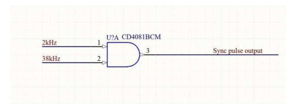
In first part we make two square pulses with function generator in 2 kHz and 38 kHz which is match to the receiver sensor and sync them in logic gate also generate with 555 timer IC [9]. Figure 13 and Figure 14.
$$F = 1.4/((R_1 + 2R_2) * C_1)$$
$$T = 0.69 * (R_1 + 2R_2) * C_1$$
$$DutyCycle = R_2/(R_1 + 2R_2)$$
$$f = 1.4/((6.8k + 2(69k\Omega) * 0.01uF = 966Hz)$$
$$f = 1.4/((120 + 2(3.566k\Omega) * 0.01uF) = 37982Hz)$$ (8)
In the receiver part, at first we design a discrete band-pass filter and test it
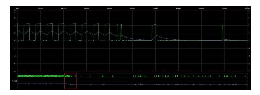
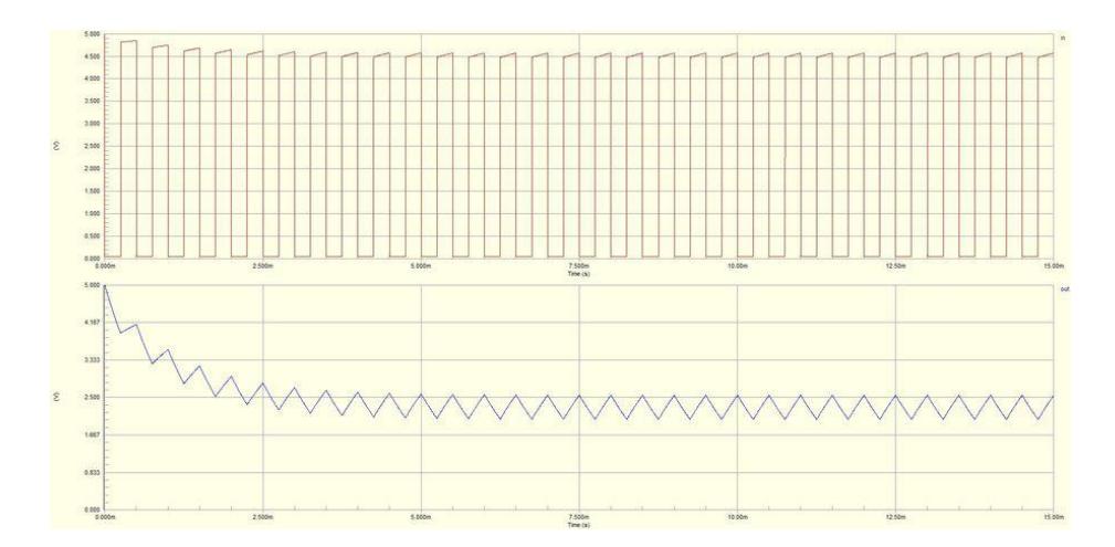
in laboratory. The ambient noise with any intensity makes an offset in receiver sensor output. So we makes an AGC [11], then the project stopped because of ignoring lots of important parameters in designing. As a result we decide to use infrared remote-control receiver modules instead of these discrete boards. These sensors square output will be 50% duty cycle by receive active infrared and 100% with infrared line, Figure 15. The resulting square digital output of sensor is sent to a RC low pass filter. The circuit is simulated in Altium designer software to calculate and choose the optimum values for capacitor and resistors of the filter. The output of this digital to analog converter is compared with a special
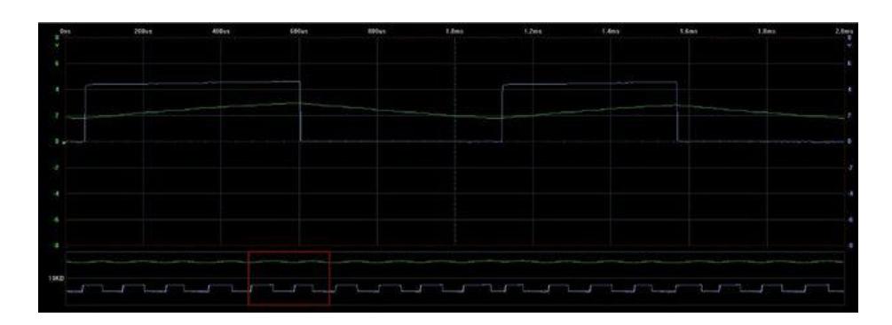
DC voltage that show us ball position as a flag, Figure 15 and Figure 16. The time constant of the RC filter is calculated as:
$$T = RC \Rightarrow 1.034ms = 4.7k \times 220nF \tag{9}$$
To protect sensors and have better ball positioning, the location and structure of sensors is changed. As the result, we have a special line sensors that provides the same ball position in every environmental conditions. This architecture faces some problems as:
- Time limitation in sensing causes delay in ball detection.
- Grand voltage a noise that is generated in starting current of motors causes some errors in the receiver circuit.
- Different voltage level compare to ARM causes some difficulties in design.
According to the drawbacks mentioned above, redesigning of this structure seems essential. Implementation of IR sensing in FPGA, eliminates these constraints with lowest software and hardware cost. Now, we are going to generate and sync transmitters pulse in FPGA and count receiver pulse in a predefined period of time.
3.4 Wireless board
According to the new small size league rules in enlargement of the field and the data packet lost problem, we decide to improve our wireless communication yield with a high efficiency wireless LAN PA, pursuant to our wireless communication module (nrf24101+), increase our signal power from 1dBm to 28dBm and change antenna from 7dBi to 11dBi.
4 Mechanical Design and construction
Typically, the main portions of mechanical structure of a small size robot, include 4 wheels, two kickers, a dribbler and the motion transformer system, Figure 17.
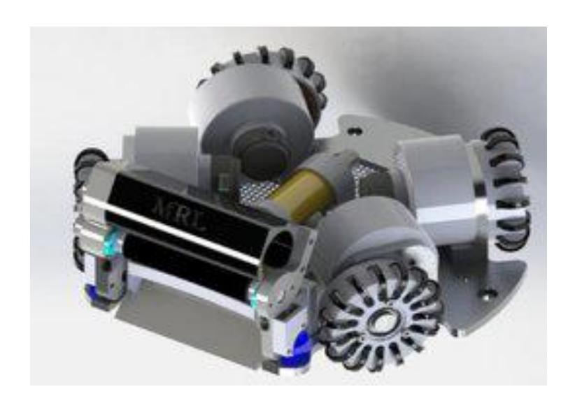
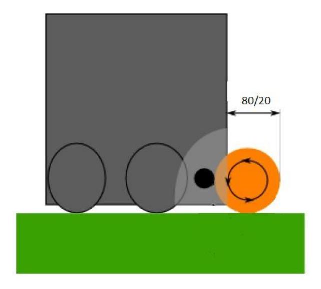
Regarding the league rules, diameter of the robot is 179mm and the height is 140mm. The spin back system conceals 20% of the ball diameter in the maximum situation.
Due to some drawbacks in the previous proposed design, we have decided to improve both the mechanical design and the construction materials. Main changes in the mechanical structure of the robot are described in the following paragraphs. The other parts are the same as 2014 robot described in [2].
4.1 Calculation of maximum ball-in-hand side acceleration
When we want to carry the ball with robot while moving to the sides, we need to know what the maximum allowable acceleration of the robot is. For this
calculation we assume that the ball is in robot by 20% of its diameter, see Figure 18.
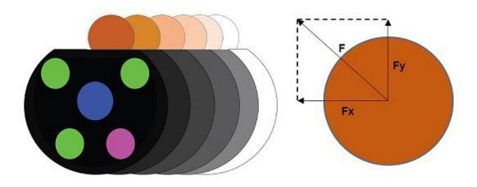
When the robot moves to the sides (left or right) a side force is acting to the ball. The direction of the force is shown in Figure 19. As mentioned, assuming that the ball is in the robot by 20% of its diameter, we have
$$F_y = \frac{12.9}{21.5}F\tag{10}$$
where
$F_y$ : Vertical section of the force F that acting to the ball.
F: The force that acting to the ball.
To analyze the force, realize that when the vertical section is greater than the force of the dribbler spin, the ball runs out of the robot. In other side, this force is calculating with the equation below:
$$F = ma (11)$$
where:
m:Mass of the ball
a:Acceleration of the robot and ball to the sides
When the robot is spinning and carrying the ball, the force to the ball is equal to the friction force between the ball and the field. So we have the following calculations:
$$F_y = F_k \Rightarrow \frac{12.9}{21.5} ma = F_k$$
$$m = 0.046kg \Rightarrow \frac{12.9}{21.5} 0.046a = F_k$$
$$\Rightarrow a_{max} = F_k \frac{21.5}{12.9} 0.046$$ (12)
where:
Fk: Motion friction force
Therefore by estimating the parameter Fk and putting it into the equation, we can calculate the maximum acceleration of the robot when moving to the sides while carrying the ball. Note that we do not calculate the vertical force in our current calculations and postpone it to the future.
4.2 Kicking systems
We use two kinds of kicking systems, direct kick and chip kick. Each kick system consist two parts, solenoid and plunger. The custom made cylindrical solenoid
is used for direct kick similar to last year which has ability to kick the ball up to 9ms. This year as a chip kicking system, because of performance problem we decided to reshape the solenoid from rectangular to cylindrical. Because of the electromagnetic effect in the cylindrical plunger two separate parts are used, one part is made from pure iron (ST37) and another one is made from Aluminum Alloy (7075). The chip kick has a 45 degree hinged wedge front of the robot which is capable of kicking the ball up to 6m before it hits the ground.
4.3 Dribbling System
Dribbling system is a mechanism to improve the capability of ball handling. As it is shown in Figure ??, dribbler is a steel shaft covered with a rubber and connected to high speed brushless motor shaft, Maxon EC16 Brushless. We examined several materials for dribbler bar, such as polyurethane, Silicon and carbon silicon tube. Carbon Silicon is selected due to its higher capability in ball handling. Since the spin back motor is in the front side of the robot, it is exposed to the strikes caused by the collision with the ball or other robots. To solve this problem, we took the spin back motors position a little back and designed a shield for it. To improve the capability of spin back to control the ball, we made a construction in which the amount damping is controlled.
Due to placing sensors transmitter in kicker system and large visibility range of the receiver which is not good for ball detecting, We decide to decrease the visibility range of the receiver sensor by creating a small 1mm diameter hole on the arm of the spin back, see Figure ??. Placing a cover on the sensors connections we save them from any unwanted damage.
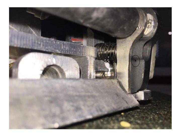
To improve the capability of spin back for ball control we made a construction in which the amount damping is controlled by two adjustment screws for proper angle and position of the spin back. The construction consists of a height adjustment screw which tunes the height of spin back structure for different carpets.
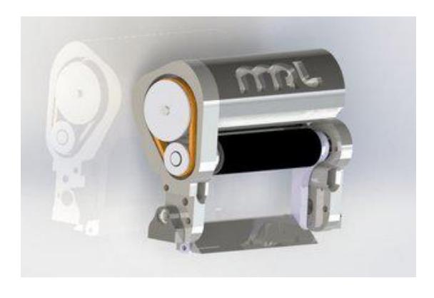
This year, we decide to replace the spin back gear box with the time belt. This leads to a better efficiency and reduces the noise of gear box. In addition, time belts are easier for installation. The best available time belt for the current structure is T2/90 because of its rate, length and pitch. The time belt properties are listed in table ??.
Table 1. T2/90 time belt properties
| Type | width length | pitch | |
|---|---|---|---|
| T2/90 | 4mm | 90mm 2mm |
References
- Ganjali Poudeh, A., Sobhani,M., H., Hosseinikia, A.,Karimpou,A., Mosayebi,S. , Esmaeelpourfard, S., Kassaeian Naeini,M. , Adhami-Mirhossein, A.: MRL Extended Team Description 2015. Proceedings of the 18th International RoboCup Symposium, hefei, China, (2015).
- Ganjali Poudeh, A., Beik Mohammadi, H., Hosseinikia, A., Esmaeelpourfard, S., Adhami-Mirhossein, A.: MRL Extended Team Description 2014. Proceedings of the 17th International RoboCup Symposium, Jao Pesoa, Brazil, (2014).
- Ganjali Poudeh, A., Asadi Dastjerdi, S., Esmaeelpourfard, S., Beik Mohammadi, H., Adhami-Mirhossein, A.: MRL Extended Team Description 2013. Proceedings of the 16th International RoboCup Symposium, Eindhoven, Netherlands, (2013).
- Adhami-Mirhosseini, A., Bakhshande Babersad, O., Jamaati, H., Asadi, S., Ganjali, A.: MRL Extended Team Description 2012. Proceedings of the 15th International RoboCup Symposium, Mexico city, Mexico, (2012).
- Ahmad Sharbafi, M., Azidehak, A., Hoshyari, M., Bakhshande Babersad, O., Esmaeely, D., Adhami-Mirhosseini, A., Zareian, A., Jamaati, H., Esmaeelpourfard, S.,: MRL Extended Team Description 2011. Proceedings of the 14th International RoboCup Symposium, Istanbul, Turkey, (2011).
- Zarghami, M., Fakharian, A., Ganjali-Poudeh, A., Adhami-Mirhosseini, A.,: Fast and Precise Positioning of Wheeled Omni-directional Robot With Input Delay Using Model-based Predictive Control. Proceedings of the 33th Chinese Control Conference (CCC), pp. 7800–7804, Nanjing, china, (2014).
- Browning, B., Bruce, J.; Bowling, M., Veloso, M.M.: STP: Skills, Tactics and Plays for Multi-Robot Control in Adversarial Environments. Robotics Institute, (2004).
- Wei, Z., Kim, B.H., Larson, A.C., Voyles, R.A.: FPGA implementation of closedloop control system for small-scale robot. Proceedings 12th International Conference on Advanced Robotics, pp. 70–77. IEEE Press, (2005).
- Texas instruments: LM555 Timer (Rev. D) data sheet. Texas Instruments Incorporated, (2015).
- Utilizing a Vishay IrDA Transceiver for Remote Control. Application Note by Vishay Semiconductors, Doc. No. 82606, (2014).
- Anbang Liu, Jianping An, Aihua Wang: Design of a Digital Automatic Gain Control with Backward Difference Transformation. 6th International Conference Wireless Communications Networking and Mobile Computing (WiCOM), (2010) .
- Gerhard Venter, Jaroslaw Sobieszczanski-Sobieski: Particle swarm optimization. AIAA Journal,Vol.41,No.8,(2003)