KIKS 2017 Team Description
Koh Ohno, Toshiki Mimura, Hayato Yokota, Tessen Ohmura, Tetsuya Sano, Masato Watanabe, Toko Sugiura
National Institute of Technology, Toyota College, 2-1 Eisei-cho, Toyota, Aichi 471-8525, Japan
http://www.ee.toyota-ct.ac.jp/~sugi/RoboCup.html
Abstract This paper is used to qualify as participation to the RoboCup 2017 small size league. Our team's robots and systems are designed under the RoboCup 2016 rules. The major points of improvement in this year are about the driving wheels, electrical circuit and AI system. The overviews of them are described.
1 Introduction
KIKS has tried to develop the robot, which mount the 70watt motors since last year. The basic design validation and evaluation was finished. The robots were manufactured and the performance was confirmed on a test run. As the results, we found many things to do and challenge [1]. Therefore, in order to solve these problems, we try to improve and redesign of the robots in 2016. It is described below as terms of the 1) improvements of robot that mount the 70watt motors, 2) redesign and manufacturing electrical booster circuit, 3) moving performance, 4) improvement of prediction of a ball.
2 Hardware design
In this section, we report the mechanical hardware of the robot.
2.1 Introduction of hardware
As reported in last TDP, we manufactured the robot, which mounts the 70[W] maxon motor for RoboCup 2016. However, there were many problems in performance of the robot. Especially, two problems were serious. One was the durability and handleability of wheel unit by directly driving, and another one was precision of straight-kicking stability by solenoid. We describe the way to fix up for these mechanical problems in below.
2.2 Evaluation of wheel built in 70 watt motor
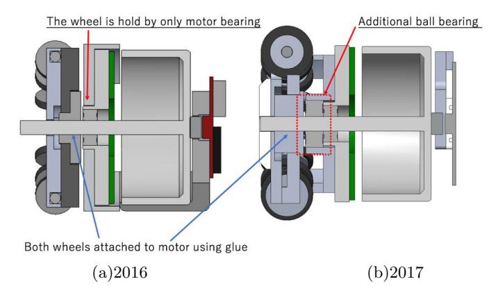
It is key point that the robot equipped with 70[W] motor is downsizing of wheel unit. Because as increasing the wheel unit-size, it will affect performance of the kicking devices. That is, the high-performance solenoid we need cannot mount on the robot. We adopted direct-driving method to drive wheels with no reducer to make motor-unit thinner. The 70[W] motor driving 48[V] producible hightorque more than that constructed through gear with the 30[W] motor equipped on present robot. Figure 1 shows the construction of direct-driving motor. In previous one shown in Fig. 1(a), it had directly load in bearing and shaft on bush of motor. Thus, we changed the construction adding new bearing to decrease the load to its own bearing in motor as shown in Fig. 1(b). The motor shaft is also directly used as wheel center even in Fig. 1(b), however, to avoid influence of external force, whole wheels are located deeply inside from outer cover of the robot.
2.3 Improvement of kicking parts
It is key point that the robot equipped with 70[W] motor is downsizing of wheel unit. Because as increasing the wheel unit-size, it will affect performance of the kicking devices. That is, the high-performance solenoid we need cannot mount on the robot. We adopted direct-driving method to drive wheels with no reducer to make motor-unit thinner. The 70[W] motor driving 48[V] producible hightorque more than that constructed through gear with the 30[W] motor equipped on present robot. Figure 1 shows the construction of direct-driving motor. In previous one shown in Fig. 1(a), it had directly load in bearing and shaft on bush of motor. Thus, we changed the construction adding new bearing to decrease the load to its own bearing in motor as shown in Fig. 1(b). The motor shaft is also directly used as wheel center even in Fig. 1(b), however, to avoid influence of external force, whole wheels are located deeply inside from outer cover of the robot. Figure2 indicates the situation of catching a ball by dribbling unit. The specification over of the robot. The specification of dribbling-unit is tabulated in Table 1. Based on the condition of Table 1 , a robot was able to catch a ball coming at about 4.5[m/s]. As the result, we found that the relationship of axes shown in Fig.2 would be one of the most efficient positions for catching and dribbling a ball. This means that the performance of newer devices are 50% better than previous one.
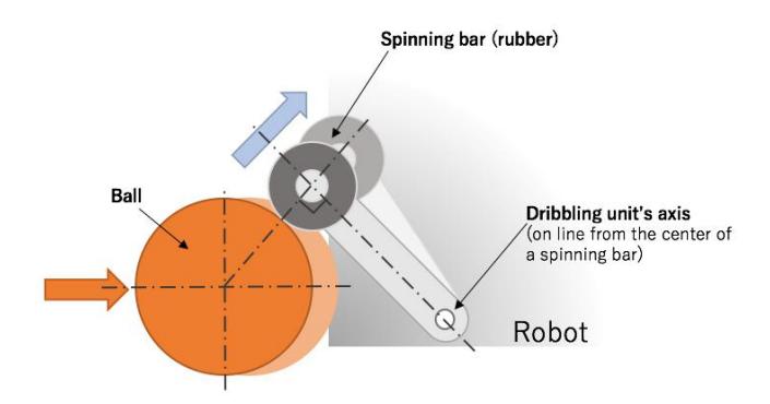
Table 1. The specification of dribbling unit
| Equipment | Detail |
|---|---|
| Motor | maxon EC max 25 watt (283860) |
| Gear ratio (in : out) | 1 : 1.4 |
| Diameter of spinning bar | 15mm |
| Material of spinning bar | polyester urethane |
2.4 Improvement of motor unit
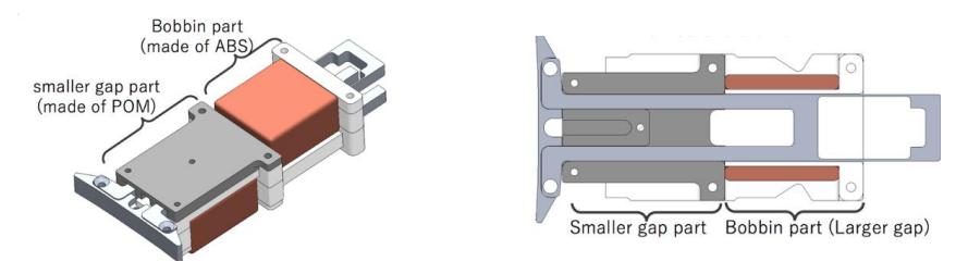
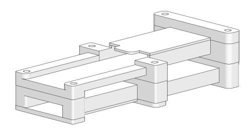
We reported that straight-kicking stability due to improvement of kicking-bar in last TDP. Its performance, however, was not enough in actual game. Thus, to increase more accuracy of the stability, we tried to remake the kicking-bar and solenoid-case (square bobbin) so as not to form large clearance. The demerit of quadrangular cross-section shape of the bobbin case will be larger distort with increase of use. The motion of the kicking-bar will be suppressed even when the gap is simply narrow. Thus, as shown in Fig. 3, we separate into two parts, i.e., small-gap part and solenoid-bobbin part to bring a solution to smooth motion and accuracy. Naturally, they are made from different suitable materials, e.g., POM resin is used for small-gap part and ABS resin is used for bobbin case. This structure made it permissible for distort of bobbin and possible to shoot with high accuracy for straight-direction for a ball. To manufacture these parts in fact, we decide to use 3D printer to reduce a volume of solenoid-bobbin. The structure is shown in Fig. 4.
2.5 Improvement of motor unit
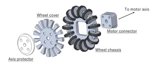
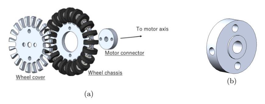
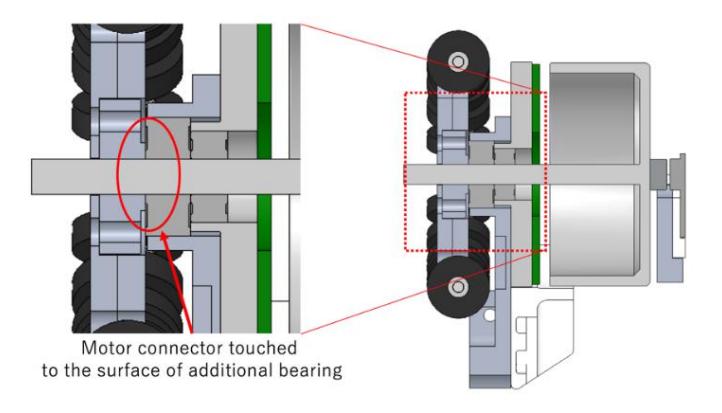
As mentioned above, the previous motor-wheel unit has lacks of handleability for maintenance and expansion. It is thought to be due to fix with an adhesive and to be incompletion of the wheel structure. The problems caused by adhesive are that the deconstructions of motor-wheel unit to pieces are difficult, or there are quite times to demount them. Applying heat to the adhesive is effective to deconstruction, but it gives serious damage to motor-axis and bearing. Thus, we should not apply it to them so often. Moreover, even happening of accidents in a game, we cannot rebond them because of adhesives need 5 hour to 1 day to be harden. In previous wheel structure, the wheel chassis was hold with only wheelcover to motor-connector as shown in Fig. 5. That was, it might cause that the small tires would drop when a motor-cover was remove and/or attached again. In addition, it will take up so much of our time to preparation. To solve these problems, we redesigned the wheel structure. The wheel cover and chassis was screwed as shown in Fig. 6(a). A new motor connector shown in Fig. 6(b) was made from A2017 aluminum with 5[mm] thick. It will be very important for the precision about center-hole's diameter and verticalness. Now, we cannot say permissible range of them by lack of measurement, it has adequate strength to motor axis even when the hole is little bit bigger than motor axis. As the results, new wheel unit is a few mm thinner than previous one. Furthermore, the bracket of new wheel-motor unit makes constantly contact with the innerring inside of bearing as shown in Fig. 7. This makes no coming off the motor-shaft even in case of adding heavy load for axial direction. We found that the distortion of motor-housing occurred in initial version model did not break out. Now, it is designing based on better plan mentioned above. The verification is not sufficient. We should manufacture the complete version as soon as possible for the RoboCup2017.
3 Electrical design
3.1 Problem of the battery for Robot built in 70watt motor
A robot needs the 50[V] to drive 70[W] motor. In fact, however, it was impossible to mount 12cells-44.4[V] lithium polymer (Lipo) battery on our robot. Because the battery size is larger than that of 4cells. In last year, due to temporal limitations, there was a highest priority to drive a 50 watt motor with minimal circuit changes. That is, we could not have enough time to establish the process of generating 50[V] using boosting circuit. So, we tried to use two 6cells-22.2[V] Lipo batteries with series connection. Nevertheless, it gave rise to some problems. First, it could not put the battery-pack into robot, yet. It is the results of the limitation of body design. Next, it is necessary to monitor the voltage by each battery-pack. Moreover, the performance of two battery using series connection need nearly equal. Thus, to deal with these problems, we redesign and manufactured a new booster circuit.
3.2 Booster circuit
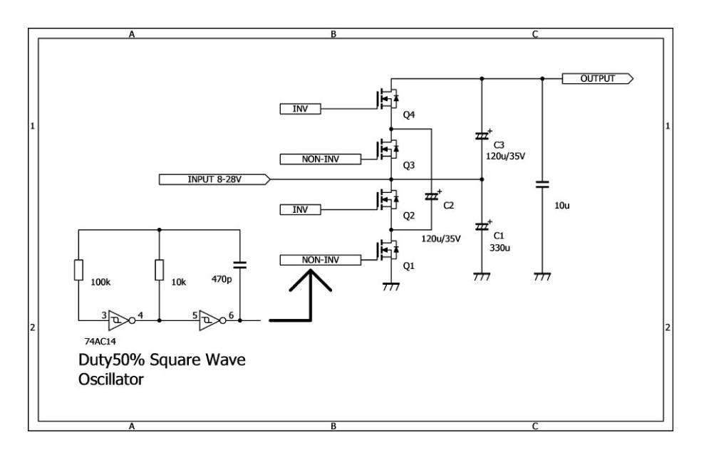
Booster circuit is shown in Fig. 8. It is known as the charge-pomp circuit or switched capacitor circuit. The charge-pomp circuit does not need the feedback of output voltage. The boosting is done by the capacitor which charged to the same voltage as the battery is connected in series with the battery by switching. Depending on the circuit construction, it will be feasible three times for the input voltage. However, it is impossible that the capacitor voltage is higher than battery voltage in this case. So, no more than over double voltage of the battery will be output. In the case of break down for booster circuit, the considerable main reasons are breakage of switching FET and/or charging capacitor. If FET is broken in short mode, battery may be shorted with GND. But, since fuse is inserted to input side, the circuit will be shut down mandatorily. Furthermore, it has less incidence of magnetic noise by no use of inductor. Alternatively, it need large capacitor against large current overload. We use the conductive polymerelectrolytic capacitor for it. We notice that input current will be larger than that of output in booster-circuit.
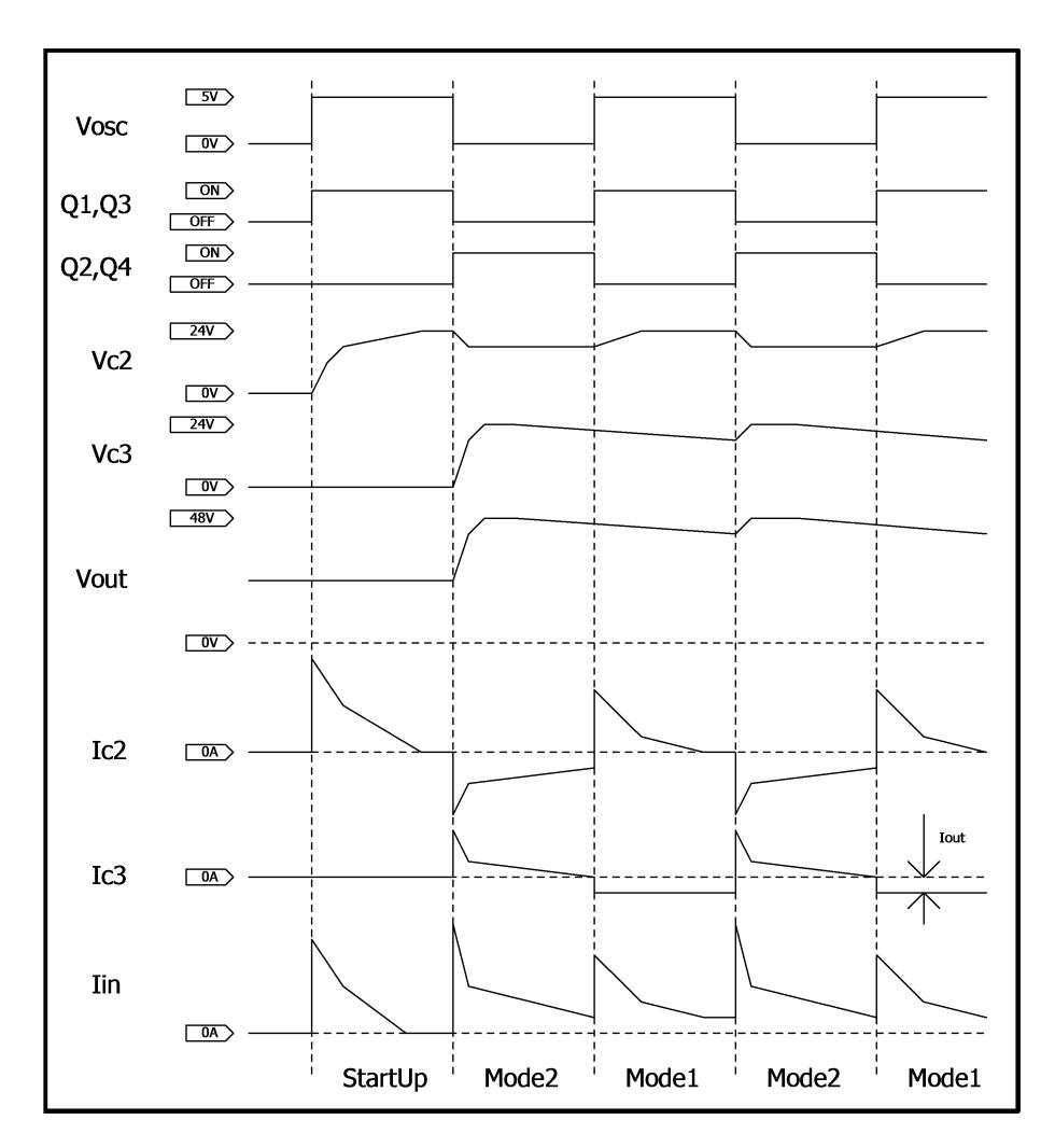
3.3 Behavior of booster-circuit
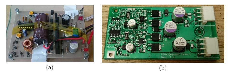
It explains the booster-circuit behavior by use of time-chart shown in Fig. 9. As the action of circuit, mode1 and mode2 are alternately actuated. In mode1, $Q^1$ and $Q^3$ are on-state. Then, $C^2$ is charged up from battery pack, and the voltage between terminals $Vc^2$ is raise up to 24[V]. In mode2, $Q^2$ and $Q^4$ are on-state. Then, $C^3$ is charged up by $C^2$, and the voltage between terminals $Vc^3$ will result 24[V]. Because of output voltage is sum of input voltage Vin (=24[V]) and $Vc^3$, $Vout$ is approximately 48[V]. After that, $Q^1$ and $Q^3$ will be on-state again, and $C^2$ is also charged up by power supply. Since $C^3$ keep the voltage, $Vout$ also keep about 48[V]. Thus, if the switching stops, output voltage won't fall down below input voltage. That is, it means that it will be very dangerous on case of electrically shorted. Similarly, it also risky for sudden short-circuit fault of $Q^1$ and $Q^2$. Therefore, it should insert the fuse to input stage of circuit. Figure 10 shows the booster circuit. Prototype version shown in left side cannot use on the actual game, but it is for checking and evaluation for operation. Actual mounted version is shown in right side. It is manufactured smaller than prototype version.
4 Software design 1 -Robot control-
4.1 Improvement of the running performance (slip suppression)
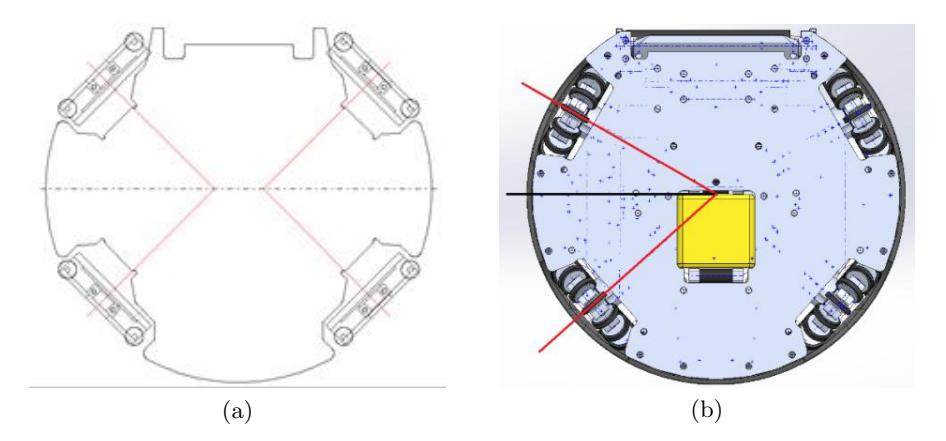
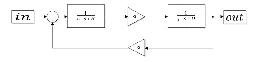
In last year, we manufactured new robots, which equipped 70watt-motor for their wheel motor. The solenoid, dribble unit and so on were also remade. The most significant change is the improvement of wheel's layout. In previous robot, the axles of each wheel did not across the center of robot's bottom, and no axles connected to that of corresponding opposite side as shown in Fig. 11(a). On the other hand, the new one shown in Fig. 11(b) indicates that all axles across and connect on the center of the robot. In addition, the longer distance between front wheels than that of rear will give dribbling-unit an advantage. By this improving, the running stability for back and forth was increased. A dribbling-unit could be also wider because the front space was enlarged. We have used these robots since RoboCup2016. In a game, we evaluated about these improve-ments, and confirmed the effectiveness of enlargement of dribbling-unit for performance of catching a ball. As the result, it would be easier to catch and to shoot a ball passed from an ally robot. However, the performance of braking and moving in diagonal direction would not be better. That is, the changing of wheel-layout was not bring the all performance of the robot. It attributed the worse performance to the asymmetrical layout of wheels. It might be caused by slipping of wheels notably in moving. Therefore, we try to improve the running performance with suppressing the slipping. In general, it is valid to introduce a feedback (FB) controller such like this case. It is also useful to design the electric current controller to get fast response to the motors. Thus, we considered how construct the control system including the current feedback when wheels slip. We use three-phase DC brushless motor to drive wheels in robot. The three-phase ($uvw$-coordinate) system is able to convert to two-phase ($dq$-coordinate) system. Then, the torque of wheels is only depend on $q$-current, while $d$-current affect only magnetic field. Therefore, with merely focus on the $q$-current, the behavior of three-phase DC motor will be able to replace with that of single-phase one. Hereafter, we discuss as single-phase DC motor about the current behavior in slipping state. The circuit and mechanical equations of DC motor are given as following eq.(1). These equations about DC motor displays as the block diagram shown in Fig. 12.
$$V - k_E \omega = L \frac{dI}{dt} + RI$$
$$\tau - k_\tau I = J \frac{d\omega}{dt} + D\omega, \quad where, \quad k_E \approx k_\tau$$
When a wheel slip, the wheel do not touch the ground and the motor-torque does not sufficiently transmitted to the wheel. Then the load of motor decreases and revolution speed increases drastically. This process of slipping can be explained as a decreasing of moment of inertia. When the revolution speed increases by slip, a counter electromotive force gets larger. After that, output would be decreased as increasing of counter electromotive force. The decreasing of electric current caused by slipping provides feedback to the controller, and this current will increase to follow the command value. Finally, input voltage also become bigger and revolution speed gets faster and faster. If the current FB controller is simply constructed, the revolution speed get faster by slipping and it may cause serious damage to the robot. Thus, instead of FB controller, we consider the feedforward (FF) controller. In this case, since the current does not follow the command value, the increase of input voltage is smaller than that of FB controller. Therefore, the increasing of revolution speed caused by slipping will be suppressed and the effectiveness to the slipping may be indicated. The decreasing of current and/or torque caused by counter electromotive force is known as torque (current) drooping. The current FF controller with torque-drooping will be able to suppress the slipping of wheels.
4.2 Analysis of FB and FF controller using MATLAB/Simulink
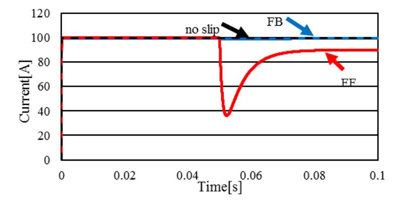
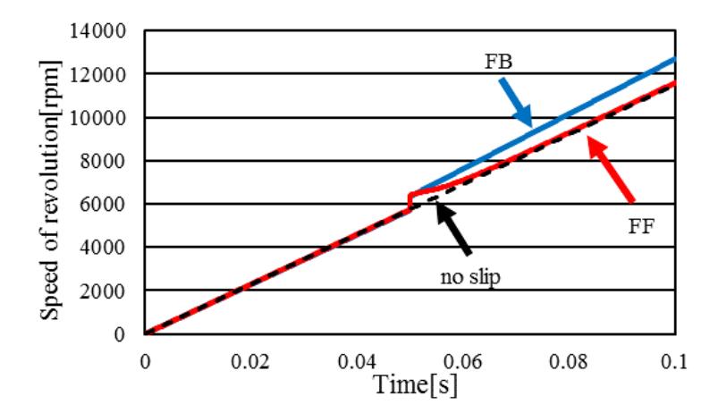
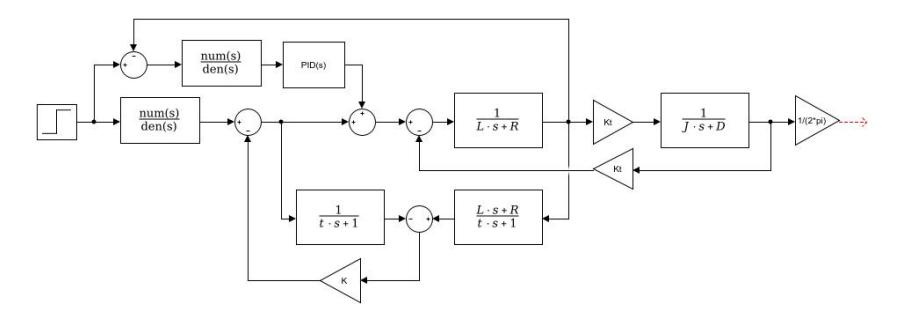
To confirm the difference between behavior of the FB and FF controller, we simulated by use of MATLAB/Simulink. The tracking performance of current and speed of revolution in each control system for target constant current shown in Fig. 13 and 14, respectively. In Fig. 13 and 14, it suppose that the slipping occurs at the time when the revolution speed increases instantaneously. According to Fig. 13, when the slipping occurs, the current in FB controller was following target value as with no slipping. On the contrary, the current in FF controller decreased as increasing the revolution speed. Moreover, in FB controller of Fig. 14, the revolution speed rises away from the line of no slipping. On the other hand, the revolution speed of FF controller keeps the line of no slipping. Summarizing the results, it found that FF control could suppress the abnormal rising in revolution speed seen in FB controller, i.e., FF controller using torque drooping was effective for suppression of the slipping. In this paper, we focused on FF control. In case of applying to actual game, it is not enough for only FF control because of there is no target followability for use of applications with many disturbances. Thus, we propose 2-degree-offreedom control system with FF and FB controller to realize the suppression of slipping with keeping target followability. In this method, but, it might be difficult to give the appropriate gain for FF and FB controller. In steady state, it requires the high-performance of target followability, while in case when the slip occurs, it requires the large effect of torque drooping. Thus, we consider implementation of the disturbance observer. It will be able to adjust torque drooping by estimating the counter electromotive force by use of disturbance observer. As the results, we think that it will be able to obtain good performance of slipping-suppression keeping target followability in steady state. Now, we do not implement the disturbance observer yet. However, we have a plan to simulate a 2-degree-of-freedom control system containing disturbance observer as shown in Fig. 15 as soon as possible.
5 Software design 2 -Receiving a ball-
5.1 Introduction of software design 2
The robot has to accurately catch the ball, and shoot to goal quickly. Nevertheless, even now, we cannot catch the ball correctly in robot because of poor prediction of AI system. In AI system, it has used Kalman filter, however, the data are processed with no pretreatment. So, the prediction had inadequate accuracy. Thus, we try to change the process of calculation for ball's velocity. It is shown in below the improvement that carried out to obtain better information.
5.2 Improvement of prediction for ball's velocity
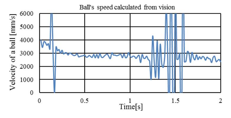
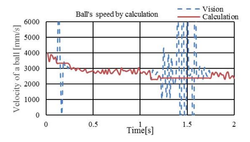
In SSL vision, only position data is able to get from vision system. Thus, we have to derive the ball's velocity using somewhat filtering process. Because of the error in observation, simple calculation between present and previous positions cannot use directly as the information of the velocity. Typical calculated velocity of a ball is shown in Fig. 16. It is shown that the speed of the ball gradually decrease in Fig. 16. We can find significant change of the speed around 0.2[sec] and 1.5[sec] obviously, such like 6000[mm/s] or 0[mm/s]. This is due to no or much difference in a sequential frame data. It is very important to increase the precision of past data for future prediction. So, we tried to make a smoothing-process using arithmetic average and variance for calculated velocity of a ball. The average and variance of ball's velocity for some frames are calculated. When the present variance exceeds the past variance, the present data is excluded and replaced to past data. The result applied the process is shown in Fig. 17. The red solid-line shows the results of arithmetic average and variance for five frames as an example. It is found that rushing noise caused by simple calculation is suppressed. We adopt this procedure.
5.3 Prediction for a ball
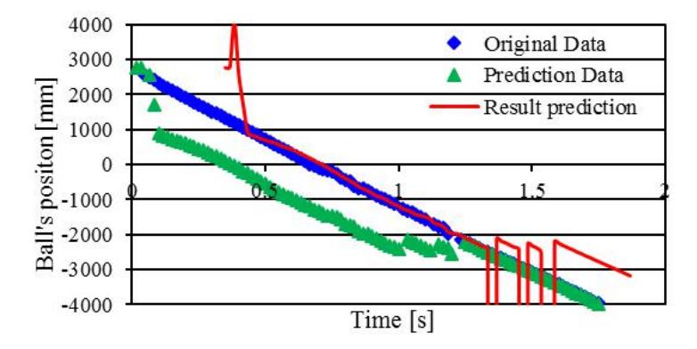
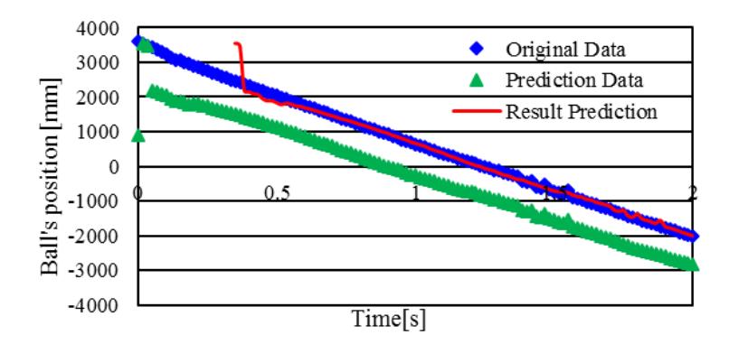
Up to now, we have made a prediction for a ball, and used for passing a ball by aid of Kalman filter in RoboCup competition. Nevertheless, its performance is not enough. To improve the predictive performance is necessary step towards getting high in ranking. We assume that ball's acceleration is attributed to friction of kinetic and air. Under the condition, we predict the future behaver for a ball. In previous prediction, we made a prediction on the assumption that a ball speed was linearly decreased. The decreasing of the velocity of a ball in fact, however, will be nonlinear corresponding on the field [2]. It often causes much disagreement between actual and predictive value. The result of prior estimation where a ball will run in about 330[msec] before-hand is shown in Fig. 18. In Fig. 18, it is only plotted for coordinate of $x$-axis. The blue diamond (◆), green triangle (▲), and red solid-line show the ball-running data, prior estimation data 330[msec] beforehand, and shifted result for green triangle data, respectively. Even in previous system, it found that future prediction will be done. However, the smart estimation is not achieved as seen around 1.5[sec] in Fig. 18, because of the influence of rushing noise as shown in Fig. 16. Thus, we try to apply the process for Kalman filter as mentioned before, and we evaluate the predictive performance of a ball position with the conventional method. The similar experimental findings to Fig. 18 is shown in Fig. 19. The red solid-line shows better agreement with the actual position for a ball compared with Fig. 18. This reason is due to the effect of smoothing pretreatment for the velocity of a ball. But, in initial time around 85[msec] (necessary time for smoothing processing), it cannot make enough estimation. The difference between actual position and prediction value is within the $\pm$40[mm] precision which allowable error. That is to say, it shows that the position of a ball is able to estimate in 100[msec] beforehand with satisfactory accuracy.
5.4 Catching performance for passed ball
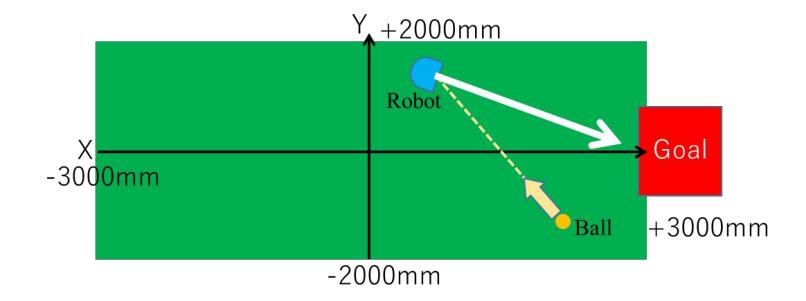
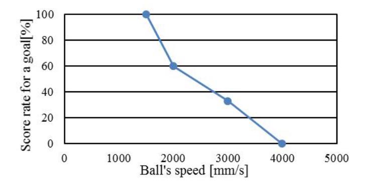
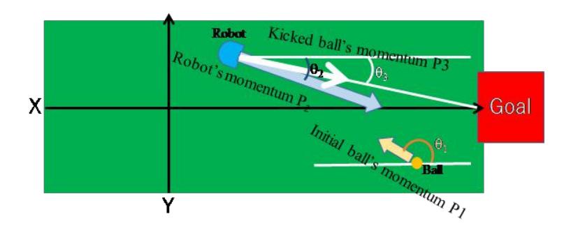
Next, we check the catching performance using two actual robots. On the field of 4000[mm] × 6000[mm], the ball is kicked from position coordinate ($x, y$)=(2275, 1460) by a robot to another catching robot's location ($x, y$)=(500,1500) as shown in Fig. 20. We repeated this experimental process five times. Similarly, changing a ball's speed and compared the success rate to goal. The results are summarized in Fig. 21. Figure 21 indicates that the score rate for a goal will be perfect when a ball's speed is below 1500[mm/s]. On the one hand, the score rate decrease with the increasing ball's speed. Now in this experiment, when the robot receive a ball, the angle and direction of robot to a goal is determined to focus the center of goal posts with no dependence on ball's speed. As increasing a ball's speed, however, momentum of a ball is increased. Therefore, it should be consider an actual momentum. It may causally relate to inconsideration of momentum of a ball as shown in Fig. 22. $P_1$, $P_2$, and $P_3$ show the magnitude of momentum vector for passed ball, kicked bar on robot, kicked ball to goal, and $\theta_1$, $\theta_2$, $\theta_3$ are defined as the angle between side-line and direction of each momentum vector in Fig. 22, respectively. By the conservation of momentum, it is calculated according to the following eq. (2).
$$\overrightarrow{P_1} + \overrightarrow{P_2} = \overrightarrow{P_3}$$
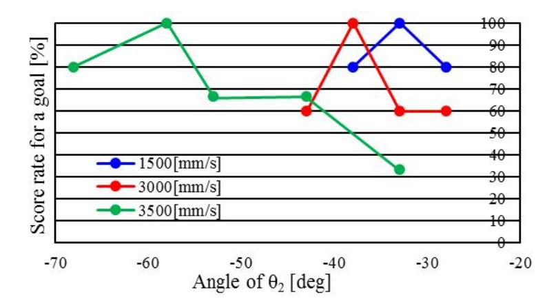
Equation (2) means that $\theta^2$ is not equal to $\theta^3$ in obvious. Up to now, our team did not take into account this factor, i.e., assuming that the momentum of passed ball was much smaller than that of the kicked bar, it might be ignorable. As increasing the ball's speed, however, it cannot ignore naturally. We think that this is the reason for the worse result in higher speed shown in Fig. 21. So, we investigated again the score rate of a goal with respect to $\theta_2$, as changing a ball's speed, but $\theta^3$ is fixed as -33[deg]. The results are summarized in Fig. 23. As shown in Fig. 23, it found that even under the condition of over speed 1500[m/s] for a ball, score rate for a goal was raise up. Furthermore, it was confirmed that there was the optimal value depending on a ball's speed. Its value roughly satisfied to $\theta^2$ given in eq. (2). When the robot's performance will improve hereafter, some characteristics may be changed. Thus, we should introduce appropriate parameter to preset AI system as soon as possible. Moreover, as future tasks, we need to think about the prediction from ball's momentum and robot's position for opposing team's tactics. In addition, it is also issues that estimating some parameter to use filtering and prediction system from data analysis in playing game in future.
References
- T. Sakaguchi, K. Ohno, T. Mimura, N. Tanaka, K. Satoh, Y. Yamauchi, Y. Nagasaka, M. Watanabe and T. Sugiura: KIKS 2016 Team Description, http://www.ee.toyota-ct.ac.jp/~sugi/RoboCup.html
- Piyamate Wasuntapichaikul et al.; Skuba 2010 Extend Team Description, http://wiki.robocup.org/File:Small Size League - RoboCup 2010 - ETDP Skuba.pdf