MCT Susano Logics 2017 Team Description
Kazuhiro Fujihara, Hiroki Kadobayashi, Mitsuhiro Omura, Toru Komatsu, Koki Inoue, Masashi Abe, Toshiyuki Beppu
National Institute of Technology, Matsue College, 14-4, Nishi-Ikuma, Matsue, Shimane, 690-8518, Japan
Abstract MCT Susano Logics have been taking part in the RoboCup Japan Open since 2011 and in the international RoboCup since 2013. This year, we rewrote our AI software in Python to shorten the coding time and to acquire adequate performance test time. We adopt a Kalman filter to eliminate statistical noise, to estimate lost samples, and to compensate for the delay of SSL-Vision. The chassis of the robot was modified to improve the linearity of the moving of the robot.
Introduction
MCT Susano Logics was founded in 2011, and the team was named after a hero of Japanese mythology, Susano-no-mikoto. Susano-no-mikoto was a brother of Amaterasu, the goddess of the Sun, who exterminated a huge dragon, which had an eight-forked head and an eight-forked tail. Our team was named with the hope to win against strong and intelligent dragons in SSL.
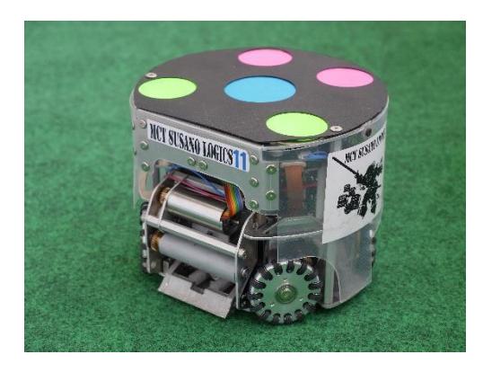
Susano Logics have been taking part in the RoboCup Japan Open since 2011 and in the international contest, RoboCup, since 2013 in Eindhoven, Netherlands. Our robots have a distinctive transparent shell (Fig. 1), but the specifications of robots and performance of AI are not at all outstanding. This year, we improved both our software and hardware. We rewrote the AI program to shorten the coding time and to acquire adequate performance test time. The chassis and omni-wheels of the robot were modified to improve the acceleration and linearity of the robot moving. This TDP describes these improvements.
Software Structure
Overview of Control Software
From our team's start in 2011, Susano Logics' control software had been developed in C++ language. C++ is a suitable language for system programming and the performance, efficiency and flexibility of it are strong. However, it requires discipline to understand and code, so it is difficult for new team members.
We decided to change the AI code from C++ to Python 3 in 2016. We adopted Python for programming AI, because its syntax allows programmers to write clear and highly readable codes. Frequent additions or alterations of code are required to improve AI. Adequate program tests after the additions or alterations are necessary for software development. However, we spent a long time for creating C++ code. The shortage of development time resulted in inadequate program tests, therefore, unanticipated situations (e.g. SSL-Vision's misreading of a robot ID) caused our AI to go out of control during games. Improved productivity brought by Python bring us much more time for testing the code, which would reduce bugs.
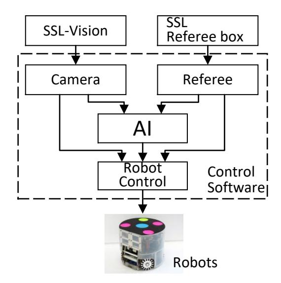
Figure 2 shows the structure of our control software. The program consists of four modules of referee, camera, AI, and robot control. The allows in the diagram of Fig. 2 indicate the data flow between the modules; the referee and camera modules are the publishers, and AI and robot control modules are subscribers. The camera module receives robots and a ball X-Y coordinates from SSL-Vision, and uses a Kalman filter to eliminate statistical noise, to estimate lost samples, and to compensate for the delay of SSL-Vision. Then the module publishes filtered coordinates to AI and robot control modules. The referee module gets commands from the SSL referee box and publishes it to the AI and robot control modules. The robot control module calculates the direction and speed of the robots from coordinates, which are determined by the AI module. The module limits the robot speed while the referee module sends stop game mode.
Behavior Tree for the AI Module
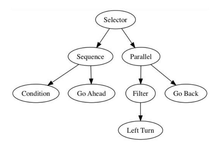
We are now programming our AI with behavior trees [1]. Behavior trees is a popular method for creating game AI, which uses nodes to select and execute robot commands. Figure 3 shows a part of our behavior tree. The program starts from the top (root) of a tree, then checks each node from the left first. In the example of Fig. 3, a process starts from the top selector, which selects a play. Then the AI executes the sequence, condition, go ahead, parallel, filter, left-turn, and finally, go back. Branch nodes (sequence, parallel, filter) select tactics for child nodes. Leaf nodes (condition, go ahead, left-turn, go back) select commands to robots. Each node has a state of success, failure, or running. For example, the branch node sequence executes child nodes of condition and go ahead, until all child nodes reach a failure state. Condition nodes check the availability of intercepting the ball. When the state become a "success", the AI sends an intercepting command to a robot.
Since Python is an interpreted language, programs require a relatively long processing time. Our AI have not succeeded to handle 6 robots within a control interval of 16.7 milliseconds on a Dell Inspiron 15 5000 (CPU: Intel Core i7-5500U 2.4GHz, memory size: 8GB) with Linux OS (Xubuntu 14.04). We are now trying to shorten the processing time. We gave up using our multi-particle filter [2], because the filter consumes more than half of the control period. So we adopt Kalman Filter for the ball and robots position estimation.
Kalman Filter for Camera Module
A Kalman filter is an algorithm that estimates the belief at time from a series of measurements and a state model.
$$\begin{cases} x(k+1) = f(x(k)) + bv(k) \ y(k) = h(x(k)) + w(k) \end{cases}$$
Where is the system function, is the observation matrix, is the constant vector, is the system noise, and is the observation noise. The output () shows the coordinates of the ball position [Px,Py].
A four-dimensional state vector x indicates the coordinates of the ball position [Px, Py] in millimeters and ball speed [Vx,Vy] in meters per second.
$$\mathbf{x}(k) = [P_x(k) \quad P_y(k) \quad V_x(k) \quad V_y(k)]^T$$
A system model for the filter is:
$$\mathbf{x}(k+1) = \begin{bmatrix} 1 & 0 & \Delta t & 0 \ 0 & 1 & 0 & \Delta t \ 0 & 0 & 1 & 0 \ 0 & 0 & 0 & 1 \end{bmatrix} \mathbf{x}(k) + \mathbf{b}v(k)$$
Time step is the control interval of 1/60 second. System noise v and observation noise w is the normal distribution with a variance of . These values were determined experimentally.
$$\sigma_w^2 = \text{diag}(0.6 \quad 0.06 \quad 11 \quad 1.1)$$
Constant was also determined experimentally at 0.1.
Time delay from transmitting a robot move command to data receiving from SSL-Vision [2], which was running on a computer (Faith Progress MT P86000N/DVR, CPU: Intel Core i5-2500 3.3GHz, memory size: 8GB) with four cameras (Allied Vision Stingray F-046C) was measured by counting the control cycles of our AI. The average delay was 6±1 cycles, which corresponds to 96±16 milliseconds. The average dead time of our robot from command reception to start moving was measured from pictures taken with a digital camera (CASIO EX-FH25) at the high speed mode of 1000 frames per second was 42.9±5.6 milliseconds. Thus, the delay of SSL-Vision was 53±16 milliseconds.
For compensating this 53 milliseconds delay, the camera module publishes compensated position estimates. The compensated coordinates cPx(k) and cPy(k) are the sum of estimates Px(k) and Py(k) and products of velocity vectors and 53 milliseconds.
$$cP_x(k) = P_x(k) + 53V_x(k)$$
$$cP_{\nu}(k) = P_{\nu}(k) + 53V_{\nu}(k)$$
Shoot Destination Prediction Filter
The prediction of a ball destination is important for the goalie to defend a goal shot. The ball arrival position is the point of intersection between the goal line and the motion vector line passing through the estimated ball position of time k. However, the motion vectors, which were calculated from the difference of an estimated ball position by the Kalman filter fluctuates widely.
To get a precise estimation, we tested three additional filters, a first-order low pass filter (LPF), a second-order LPF, and an average filter. The prediction algorithm distinguishes a kick when the ball speed increased more than 0.5 meter per second (k = 0). The motion vector of time k = 0 is not accurate, because the ball was kicked between time (k = 0) and previous (k = -1). Thus, an additional filter starts prediction from time k = 1.
The ball destination is calculated from the following equations. The input of filter, which is the estimate of Kalman filter is Py, output of the filter is P̂y, sampling interval Δt is 1/60 second, and cutoff frequency of the first-order LPF fc is 1.67 Hz.
(1st-order LPF)
$$\widehat{P}{y}(k) = \widehat{P}{y}(k-1) + \left{P_{y}(k) - \widehat{P}_{y}(k-1)\right} \frac{\Delta t}{2\pi f c}$$
(2nd-order LPF)
$$\widehat{P}{\nu}(k) = -b_1 \widehat{P}{\nu}(k-1) - b_2 \widehat{P}_{\nu}(k-2)$$
$$+a_0 P_{\nu}(k) + a_1 P_{\nu}(k-1) + a_2 P_{\nu}(k-2)$$
(Average filter)
$$\widehat{P}{y}(k) = \sum{t=1}^{k} \frac{P_{y}(t)}{t}$$
The initial values of time k = 1 are set as P̃y(k-1) = P̃y(k-2) = Py(k-1) = Py(k-2) = Py(1).
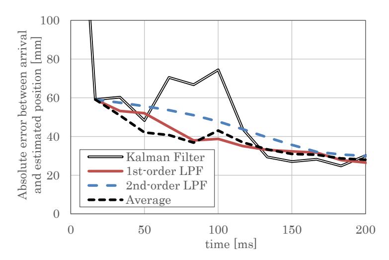
Figure 4 shows one of the simulation results when a robot kicks a ball at a speed of 8 meters per second. In order to intercept the shot, the goalie must stay within ±40 millimeters of the ball destination before the arrival. The Kalman filter output of time k=0 (0 millisecond) was over 200 millimeters, because the motion vector was not accurate as mentioned before. The filters start at k=1 (17 milliseconds). Both first-order LPF and average filter outputs converged to 40 millimeters at 83 milliseconds after the kick, but the average showed fluctuation. The response of the second-order filter was too slow. Therefore, we chose the first-order LPF for the shoot destination prediction filter.
Robot Hardware Improvements
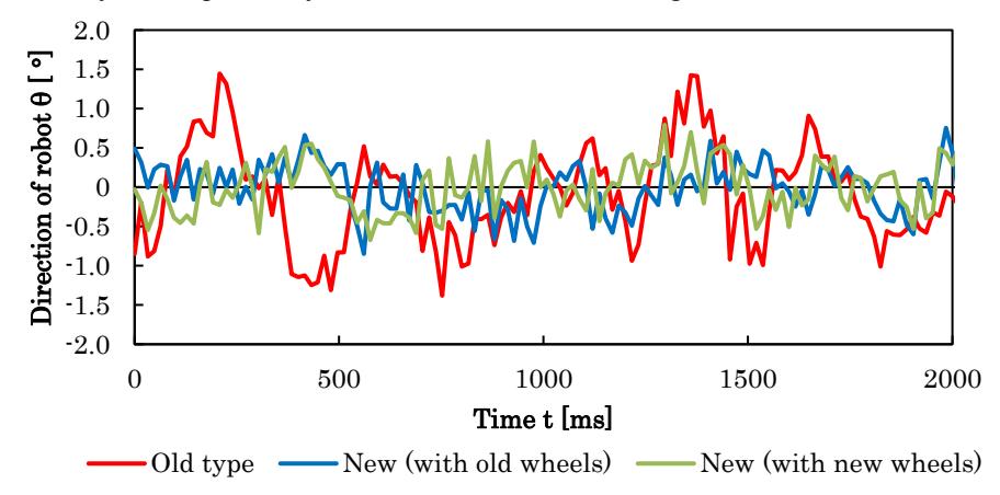
One of the problem of our robot was that the direction of movement fluctuated during low-speed driving. This phenomenon deteriorate the correctness of kicked ball direction. We thought that the touch and release of small discs around the wheel to the ground caused load change to the motors. This load change caused motor speed fluctuations. Therefore, we designed a new omni-wheel with more small discs.
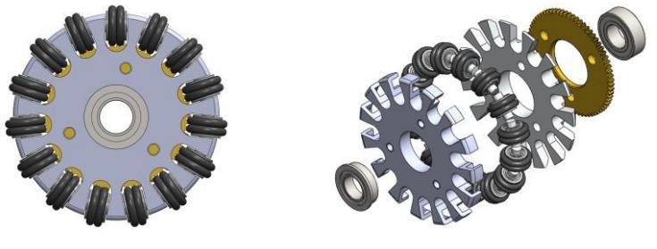
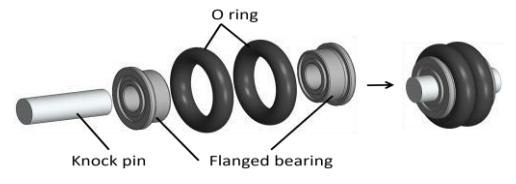
Figure 5 shows our old type omni-wheel, which has 15 small discs. The small discs were composed of two flanged bearings with two O-rings. The size of the omni-wheel is 53 millimeters in diameter, 13 millimeters in width, and 60 grams in weight.
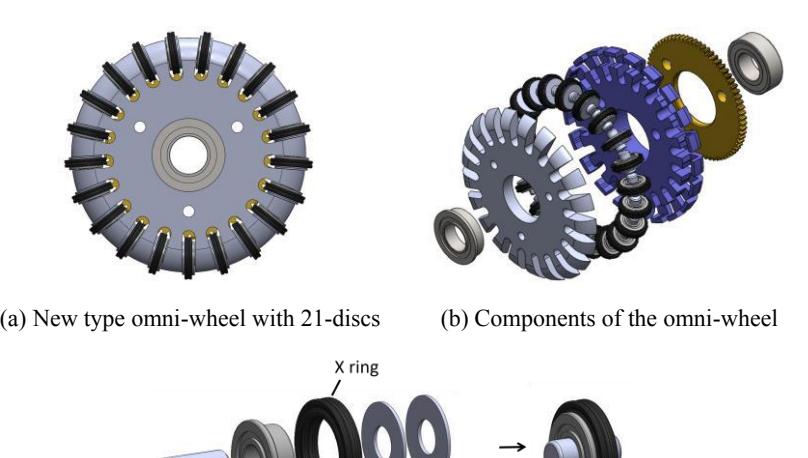
Figure 6 shows our new type omni-wheel, which has 21 small discs. The width of the small disc was narrowed to equip more discs. Therefore, the small discs were assembled from a flanged bearing, an X-ring, two washers and a knock pin. For weight reduction, inner wheel part were made from nylon. The size of the omni-wheel is 55 millimeters in diameter and 13 millimeters in width, and 57 grams in weight.
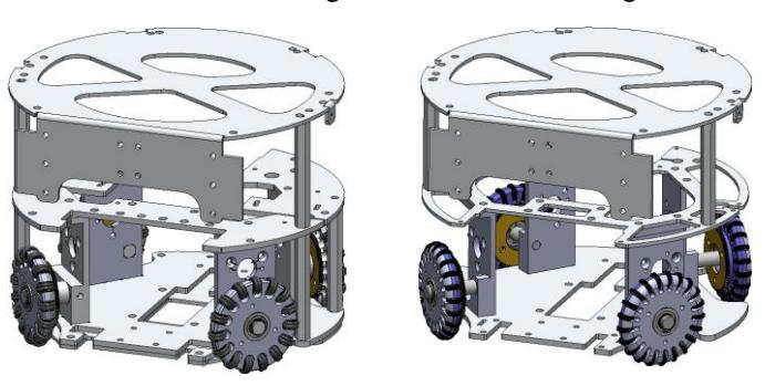
Figure 7 shows our old and new robot frames. The thickness of a bottom plate was reduced from 5 to 3 millimeters. The shape of a middle plate was optimized to support motor attachment units. The total weight decreased from 2730 grams to 2406 grams.
Figure 8 shows fluctuations in robot's directions running at our lowest speed of 0.12 meter per second. The directions of the robot were measured with SSL-Vision and the results indicated in Figure 8 were raw data from the vision. Standard deviations of a two-second running was 0.53 degrees for old robots, 0.30 degrees for new type chassis with old type omni-wheels, and 0.33 degrees for new type chassis with new type omniwheels. The new type omni-wheel did not improve the ability to hold a straight line. The ability was improved by the reduction of the robot weight.
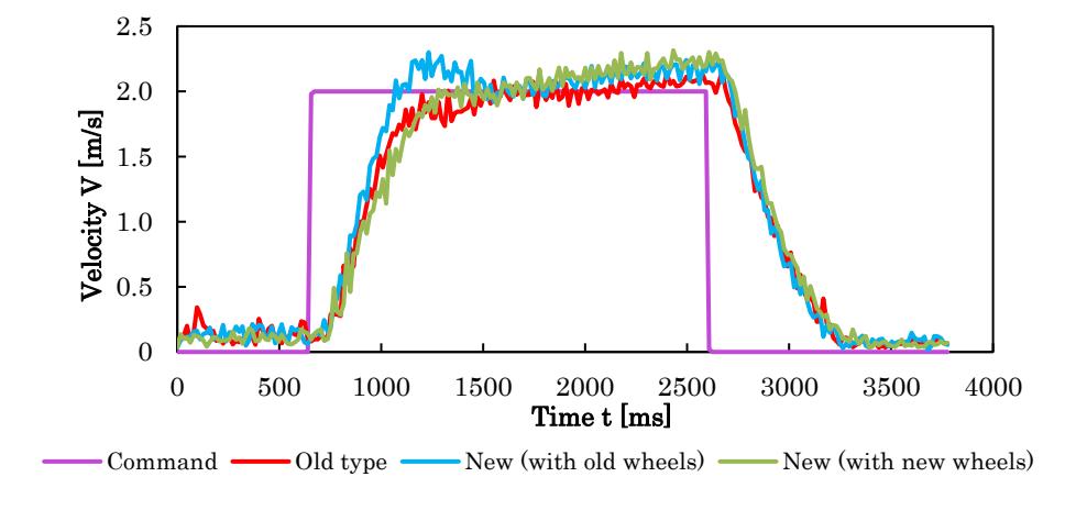
Figure 9 shows the experimental results of the robot speed from a stop to 2 meters per second. The velocities of the robot were measured with SSL-Vision and the results indicated in Figure 9 were raw data from the vision. The acceleration of the new type chassis with old type omni-wheels showed an 11 per cent increase compared to that of the old type. This is because of the 11 per cent reduction of weight. The acceleration of the new type wheel was lower than the old type. This is because of the diminution of the contact area of wheel to the field.
The new type omni-wheel showed no improvement. Therefore, we adopt the new chassis with old-type omni-wheels for the 2017 robot.
References
- I. Millington, J. Funge. Artificial Intelligence for Games. CRC Press, 2009.
- T. Beppu, S. Aoki, T. Horiuchi. A Shared Multi-particle Filter for Ball Position Estimation in RoboCup Small Size League Soccer Games. ICARSC 2016. http://ieeexplore.ieee.org/document/7781995/
- S. Zickler, T. Laue, O. Birbach, M. Wongphati, M. Veloso. SSL-Vision: The Shared Vision System for the RoboCup Small Size League. 2009. http://isites.harvard.edu/fs/docs/icb.topic859418.files/papers/sslvision2009 new.pdf