RoboJackets 2017 Team Description Paper

D. Budanov, J. Feltracco, J. Kamat, R. Medrano, S. Naeem, J. Neiger, R. Osawa, M. Pan, E. Peterson, A. Shaw, W. Stuckey, J. Ting, M. Woodward

Georgia Institute of Technology

Abstract The RoboJackets RoboCup SSL team was founded in 2007 and has competed every year since. The team's objective this year was to use the lessons learned from the previous years to rebuild the mechanical foundation, while improving the accompanying electrical and software systems. An emphasis was placed on robustness of the system as a whole. This paper outlines the progress made on the design of the fleet and the methodologies used to manifest these improvements.

1 Mechanical

The mechanical design for this year's fleet focuses on reducing the overall manufacturing time of the robot and redesigning a more reliable dribbler system. The 2017 fleet has managed to reduce manufacturing time by simplifying parts to use primarily waterjet and manual mill operations as opposed to a CNC mill.

1.1 Dribbler

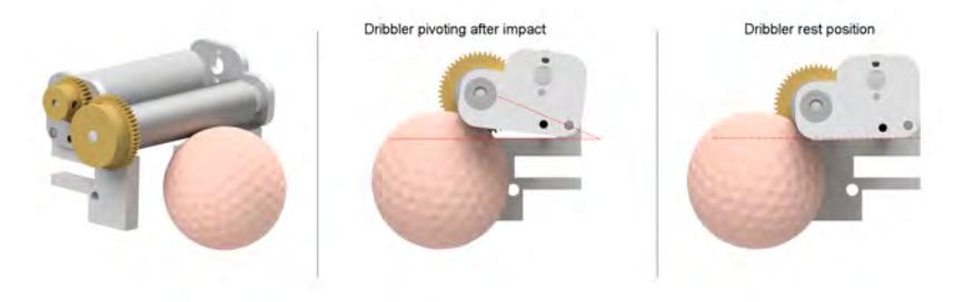
The 2017 dribbler system was redesigned based off of Carnegie Mellon's dribbler system [1]. The new design uses gravity to absorb the impact of the ball when it is initially passed to the robot, as opposed to previous years' designs that implemented a spring as the dampening system. As shown in Figure 1, the ball causes the dribbler to pivot upwards; due to gravity, it then returns to its neutral position. This new system has been tested as more efficient and consistent at catching the ball. Additionally, the new fleet implements brass gears on the dribbler system, rather than the nylon gears used in the previous year's design. The brass gears have a larger tolerance between the meshing teeth and solve the durability issues that had arisen with nylon gears. As in previous years, all dribbler system components are designed to be manufactured using a waterjet, reducing overall manufacturing time.

1.2 Motor Mounts

The 2017 fleet uses four identical waterjet fabricated motor mounts for the wheels of the robot as shown in Figure 2. This is a manufacturing improvement from last year's fleet, as previously each motor mount was CNC milled and two different motor mount designs were needed to accommodate the back and front positions. Additionally, the motor mount now supports the midplate above it as well as the base plate to improve the robot's stability.

1.3 Omniwheels

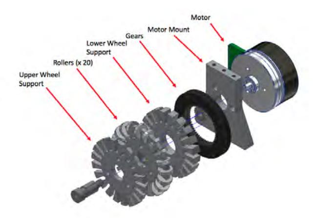
The 2017 omniwheel design is composed of three layers that constrain the rollers. Last year's omniwheel design was composed of two layers, with the bottom layer requiring a CNC operation [2]. The manufacturing time of the drivetrain was decreased by implementing more waterjet operations over CNC mill operations, as the waterjet allows for multiple parts to be cut in a single run. Previously, the manufacturing time on the CNC mill was approximately 90 minutes per wheel; now the manufacturing time using the waterjet is 60 minutes per wheel. The total manufacturing time breaks down to 10 minutes to set up the waterjet, 15 minutes to waterjet the three layers of the wheel, and 35 minutes to tap the holes in the support layer of the wheel. Additionally, due to the waterjet's ability to nest parts onto a single sheet of metal, mass production of a single part does not require any additional setup time.

2 Electrical

The electrical design for this year has focused on improving the reliability of last year's design. This was accomplished by switching radio protocols, changing the inter-board connectors, and improving PCB routing.

2.1 Ultra-Wideband Radios

The past year's version of the robot used custom radio hardware designed inhouse for a 900 MHz system. These radios had multiple issues due to the difficulty of designing custom radio hardware and firmware. The lack of reliability resulted in frequent packet loss, especially with multiple robots in use. The 900 MHz band also limited the bit rate to a maximum of 1.2 Mbps, which bottlenecked the information that could be transmitted between the robot and base station. This issue became increasingly pressing as more sophisticated control features were developed, requiring greater bandwidth between the robots and base station.

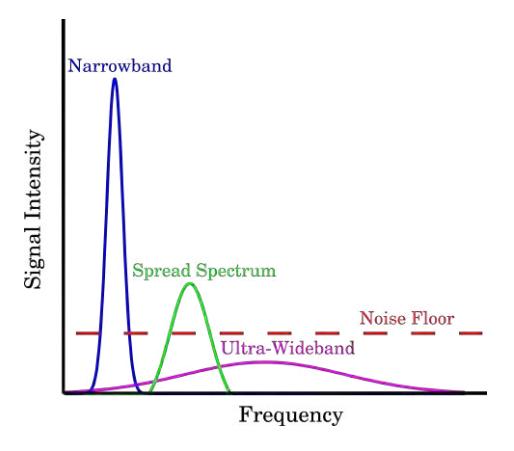
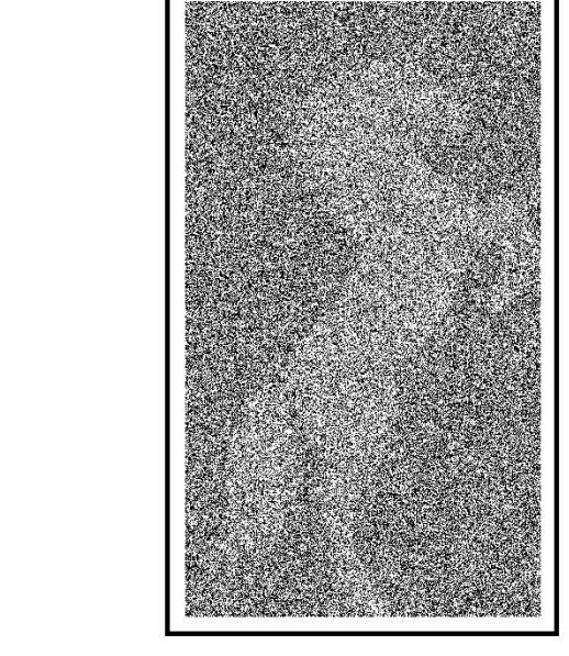
The new DecaWave radio modules use ultra-wideband impulse radio (UWB-IR) technology designed to avoid interference with traditional radio signals. The radio module transmits through a wide range of frequencies centered at 3.5 GHz at low amplitudes, therefore reducing interference with nearby narrowband transmitters and improving communication reliability. Figure 3 shows how the signal of UWB-IR stays below the noise floor, allowing for narrowband to transmit on the same frequency without interference. Detecting signals below the noise floor is similar in principle to a human's ability to detect features in a noisy image. Figure 4a is a small section of a noise-drowned grayscale image. Some gradient lines can be observed, but identifying the original image with a high level of certainty is very difficult. This is analogous to communication methods utilizing narrowband or spread spectrum techniques having difficulties accurately interpreting the received packet. The original image in Figure 4b, on the other hand, can be identified with a high degree of certainty. UWB-IR operates in a similar manner with the use of a wide range of frequencies.

The higher center frequency yields an elevated data transfer rate of 6.8 Mbps. Such higher bandwidths permit larger amounts of control and status information to be transferred between the robots and base station. The radio module contains an integrated antenna and on-board RF circuitry, allowing for easier integration into the robot and greater consistency across the platform.

2.2 Solenoids

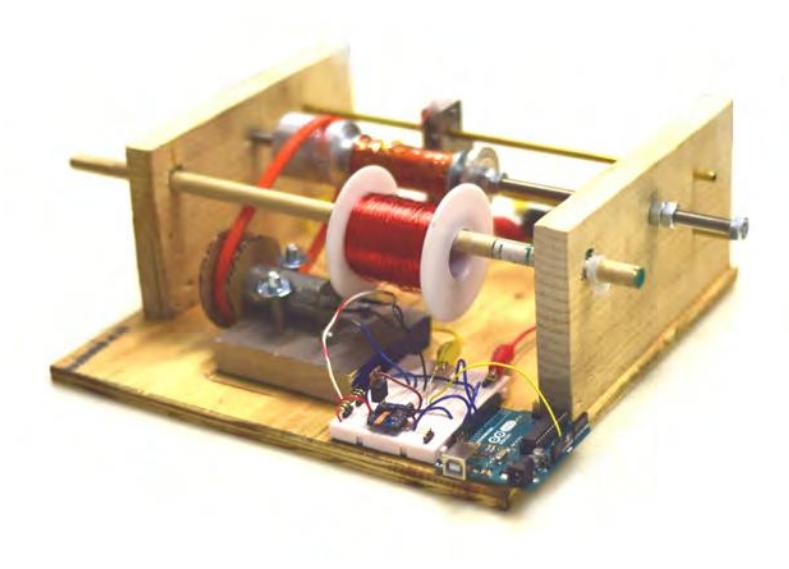
In order to experimentally determine the type of solenoid best suited for competition, a method of rapid prototyping was needed. Figure 5 displays the mechanism used by the team to produce solenoids. The mechanism consists of multiple rods attached to wooden blocks. On the center threaded rod, two aluminum spacers with tapers are pressed into the bobbin to keep it axially centered. One spacer has a groove to act as a driven pulley in the system. The spool of magnet wire used for winding the solenoid rests on the outer wooden rod, and the wire adjuster rests on the two outer brass rods. To set up the solenoid winder, a spool of magnet wire and a bobbin are placed on their respective rods. The magnet wire is then threaded through the plastic pulleys in the wire adjuster and attached to the cylinder. To wind the solenoid, a brushed DC motor drives one aluminum spacer with a belt.

2.3 Motor Board

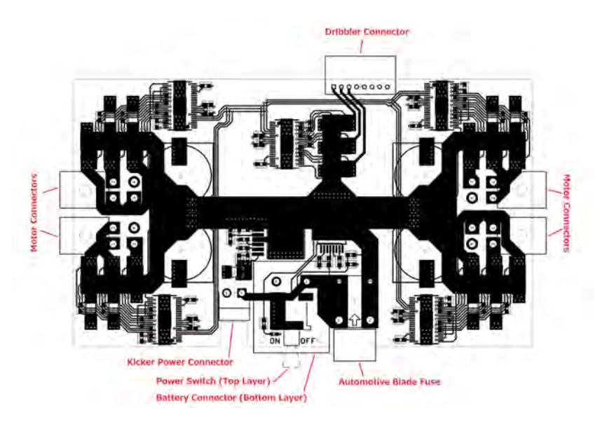
The motor board handles the primary power distribution and the motor driving functionality. The power distribution method has been changed to better separate the power and logic voltage rails. Improvements include a linearly symmetrical layout, removal of unused features, and optimization of LED indicator placement.

Figure 6 illustrates the critical components of the motor board. The primary fuse has been reverted to a mini automotive blade fuse similar to the 2011 design. This design uses the DRV8303 three-phase bridge driver to handle most low-level driver features such as cross-conduction protection and bootstrap switching controls. Commutation logic is still handled within the FPGA.

2.4 Kicker Board

The kicker board has been reworked to allow standalone operation. It features an ATtiny841 to switch power FETs to control kick power. While a control board is present, this on-board microcontroller acts as an SPI slave device and receives a command to kick or chip at a specific power. During standalone operation, onboard buttons can be used to control kicking or chipping for testing. The ADC on the ATtiny841 monitors the high voltage rail. When a kick or chip is triggered, there will be a large voltage drop; although this voltage drop cannot be used for real-time feedback, it can be used to tune the kicking velocity for future shots.

Like in previous years, the capacitor charger will use the LT3757 controller with a flyback topology. A bank of four 820µF capacitors is charged to 250V. [3].

3 Software

This year, the software team improved path planning, motion control, and high level plays. In particular, high level plays improved cohesion between offensive and defensive strategies. There were significant developments in automatic PID tuning and the RRT. Modularization of the codebase improved readability for other teams.

3.1 Probability-Based Plays

High level plays have been changed to rely more on probabilities. A game of soccer can be broken up into two major probabilities: a team's ability to score and ability to defend, represented by P(score) and P(defend) respectively. Due to the complexity of a game of soccer, it is impractical to directly calculate these probabilities, but they can be estimated through knowledge of the game itself. These estimated probabilities are further split into different attributes to simplify the implementation.

Offense P(score) is broken down into two attributes: the probability that the team can move the ball to a certain position, and the probability that the team can shoot and score from that position, P(pass) and P(shoot) respectively.

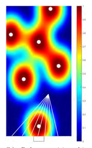
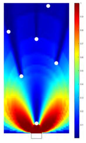
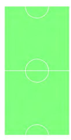
P(pass) can be calculated by estimating the error rate of the pass and mixing in the likelihood of another robot blocking it. Each opponent robot is represented as a bivariate normal distribution. The X and Y axes represent the location on the field, and the Z axis represents a robot's chance to occupy that specific location on the field. These distributions are all combined into a single 3D probability space. As shown in Figure 7b, a set of rays are cast radially from our kick position towards a goal, representing the sampled normal distribution of our potential kick. Each ray is used to estimate the chance of being blocked on that path by finding the maximum Z coordinate along the ray. This represents the probability that the kick will be blocked along that specific ray. The ray's max Z values are inverted, so the Z values represent the chance the pass succeeds along that ray as opposed to being blocked. They are then weighted based upon the kick distribution's sample value. A binary filter is applied to the resulting rays to calculate whether the ray would intercept the target segment or completely miss. Finally, the rays' values are summed together and divided by the sum of the sampled kick distribution's values. The final result represents the chance the kick will be successful and is linearly related with the actual mathematical probability of the kick succeeding. This is visualized in Figure 7c.

$$P(pass) = \frac{\sum_{n=a_{target}}^{b_{target}} (1 - \alpha(n)) \times PDF(\mathbb{N}(\mu_{kick}, \sigma_{kick}^2), n)}{\sum_{n=a}^{b} PDF(\mathbb{N}(\mu_{kick}, \sigma_{kick}^2), n)}$$

$$\alpha(n) = \max({f(r_1, \theta_1 - n) \dots f(r_n, \theta_n - n)})$$

$$f(r_{robot}, \theta_{robot}) = PDF(\mathcal{N}(\mu_{robot}, \sigma_{robot}^2), r_{robot} \times \sin \theta_{robot})$$

P(shoot) is very similar to P(pass), but there are a few notable differences. Free space is weighted more heavily when finding the best shooting position. A more accurate algorithm is used to find the largest open segment inside the goal. This is done by representing the target segment and the robot as a triangle and splitting the triangle whenever a robot is predicted to block a potential shot. Finally, the delta angle between the pass vector and the shot vector is also taken into consideration, for a more acute delta angle is much easier to act upon accurately than a larger obtuse angle.

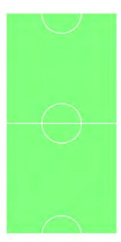
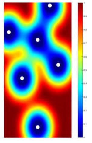
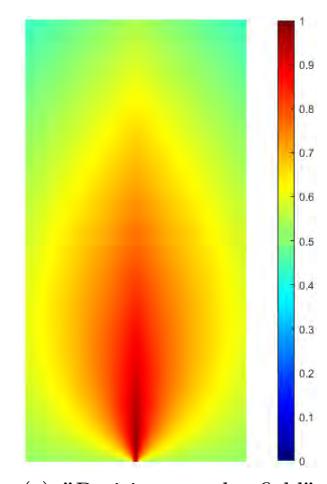
Defense Estimating P(defend) is more complex, as some of the robots' specific characteristics cannot be directly calculated. This requires a higher variance probability curve as well as some in-match automatic tuning. P(defend) is estimated through creating an opposition score for every individual opponent robot in both their current state as well as their near future state. Each opposition score is created through the weighted combination of multiple sub-scores: position on the field, shot chance, pass chance, predicted kick direction, time until activation, and angle on the ball. Position on the field is much like the one used in offense, but angle on the goal and space are weighted higher than distance to the goal. The space sub-score is shown in Figure 8b, and position on the field is shown in Figure 8c. Shot chance and pass chance are the same calculations as the ones used on the offensive side. The only difference is that opponent robots have a more accurate kick distribution. Kick direction is predicted based on the combination of the direction of movement onto the ball and the facing direction of the opponent robot. Time until activation predicts the best case time until a specific opponent robot will be able to act upon the ball. This is used to weight robots more likely to receive the ball higher. Angle on the ball represents the angle between the receive vector and the shot vector. The lower the angle, the higher this score, as it is assumed to be an easier kick.

Out of the five robots (not including the goalie), two defenders are used on the edge of the defense area to block direct shots from the ball location. To determine where the other three robots should be, score-based roles are used. The opponent robot with the highest opposition score is pressured from the goal side. The objective is to force a fumble or a pass. The opponent robot with the second highest opposition score has its predicted pass blocked with a slight weight towards blocking a predicted leading pass. With optimal blocking, this opponent robot will be unavailable as a potential pass option.

The last position uses a modified radial blob detection algorithm to find the highest opposition score area that can be defended against with a single robot. A 2D space is defined where the X axis is the angle in reference to the ball position and the Y axis is the distance from the ball. This space is used to estimate the optimal defense position. The angle axis is bucketed uniformly based on the quantity of points in that specific vertical bucket. The max bucket is found based on the total score in that specific bucket. This max bucket is the start of the area to defend. Buckets on either side of this max are added to the area based upon the derivative of the total score, as well as the absolute value as the algorithm moves to buckets on either side of the max. This produces a concrete edge on which we can split the entire 2D space into the foreground and background. The centroid of the foreground is found by treating it as a simplified 3D space with the Z axis representing the score. The resulting centroid is used as the main defense point for the third and final robot. The point is defended on the goal side with a slight weight towards the direction of the ball.

3.2 Automatic PID Tuning for Path Following

Properly tuning PID is critical to having well performing robots. An improperly tuned PID controller can lead to oscillation, slow response time, and loss of robot control. The high level motion control uses a PID controller to minimize the error between the planned path and the actual course of the robots.

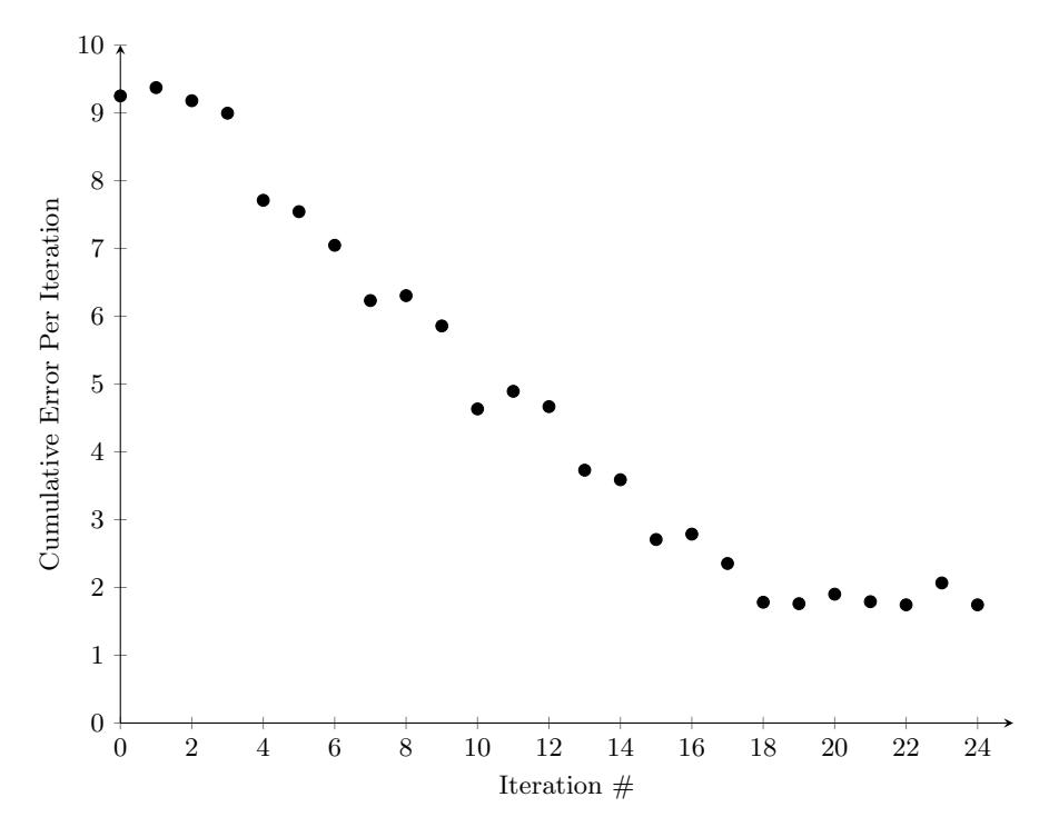
To implement automatic PID tuning, the team uses a Hill Climbing algorithm, which attempts to minimize the sum of errors while a robot is given a consistent task. The team chose to use Simple Hill Climbing [4], which maximizes the fitness score by searching the space of possible PID coefficients. In order to ensure that autotuning would be practical for use, it was important to minimize the number of iterations needed to find a maximum. To solve this problem, the space is first searched at a coarse level, and finer levels are explored later. Automatic PID tuning was integrated directly into our PID Controller module, allowing easy extensibility into other control systems, such as drive motor controls in firmware. Figure 9 shows the decrease in the error as the Hill Climbing algorithm runs.

3.3 RRT Path Planning

The team uses the Rapidly-Exploring Random Tree (RRT) path planning algorithm [2], because it can quickly compute valid paths and can easily be modified to improve its performance. Our implementation includes a 2-dimensional state space of horizontal and vertical position coordinates that is populated with obstacles. Each node in the tree represents an x-y position on the field, which builds on previous nodes in its search for the goal state.

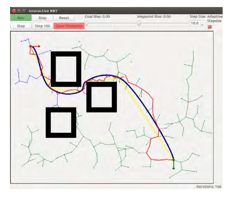
The team's RRT implementation now utilizes a dynamic stepsize inspired by Adaptive Stepsize Control (ASC) [5]. ASC is typically used in numerical analysis to limit the error accumulation of evaluating differential equations. This error control is determined by calculating an estimate of the error, and then compensating by adding an offset to the computation. When the RRT selects an existing node in the tree from which to extend, the distance from that node to the nearest obstacle is treated as the error estimate. The stepsize is then scaled based on the distance such that a small distance to the nearest obstacle results in a small stepsize, and a large distance to the nearest obstacle results in a larger stepsize, as shown in Figure 10. Taking a larger step allows us to cover more ground in the search space, reducing the runtime of the path planner. However, this can only be done when obstacles are far away, such that the increased resolution would be unnecessary.

Searching for the node in the tree to extend from is often the most computationally expensive step of the RRT algorithm. In order to determine which node in the tree is closest to the target coordinates, the RRT previously had to iterate through all of the nodes in the tree to determine which of these points is closest to the target point, which is an O(n) operation. In order to resolve this inefficiency, the team has implemented k-d trees to assist in this process [5]. A k-d tree is a type of binary tree that attempts to maintain balance by dividing the state space evenly based on the number of nodes in each partition. The branch that each node is stored under is determined by comparing that node to the median of the node in that subtree. The k-d tree is also periodically rebalanced in case an excess number of new nodes are added under the same branch. This allows for guaranteed O(log(n)) retrieval of points near a specified location, which improves the speed of the path planner.

3.4 Full Trajectory Planning

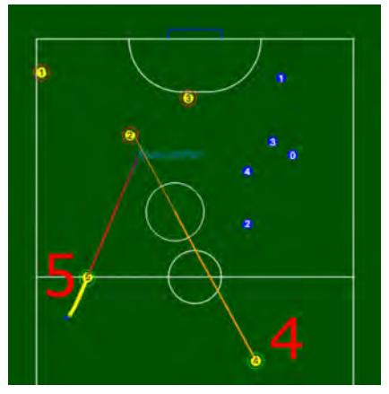
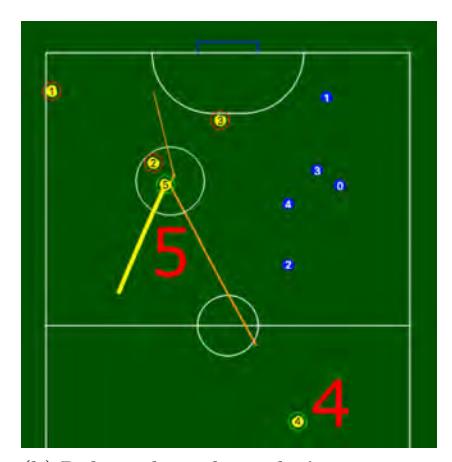
The waypoint path generated by the RRT planner is overlaid with a velocity profile in order to create a full motion trajectory – position, velocity, and acceleration at each planned timestep. The team uses a two step process inspired by the full Bézier spline motion trajectory planning in [6]. The system first creates a Bézier spline path of consecutive Bézier curves from the waypoints given by the RRT planner. It then generates a velocity path to follow the Bézier path within the robot's motion constraints. The Bézier spline path both smooths the trajectory and allow easy calculation of the instantaneous direction of movement through the first derivative of each spline. The velocity profile thus only needs to describe the speed of the robot as it follows that trajectory limited by the linear and centrifugal acceleration constraints. This was calculated with a simple linearly constrained forward and backward pass as described in [6]. The full trajectory planning system allows not only full prediction of the location and speed of each robot at all points in time, but also allows for a simple method to speed up or slow down planned paths by naively multiplying the velocity profile by a constant.

One particular use case of this was to allow full planning of robot passes, including a forward pass shown in 11a and 11b. In the forward pass, one robot kicks the ball down the field, while another robot predicts the kick trajectory and moves down the field, intercepting the ball with a line kick towards the goal. The trajectory planned for the kicking robot is naively sped up and slowed down as the predicted path of the ball is updated allowing the robot to intercept the moving ball. This separate planning of the path and velocity profile also allows more advanced velocity modification, including moving slower on delicate tasks such as aiming or avoiding moving obstacles.

3.5 Open Source and Modularity

One of the largest issues when collaborating with other teams and learning from their software stacks is inadequate modularity. It is difficult to quickly find useful information due to the complexity and size typical of RoboCup implementations; it is even more difficult to utilize them. This can be solved by modularizing the code base, making it easy for others to use and understand without dissecting an entire RoboCup implementation.

The high level software and firmware were split into two independent parts. In order to share information between parts of the software, a third project was created called common, which contains radio protocols and modules useful to both firmware and high level software, such as a time library, PID controller, and geometry library. The path planner was separated into its own project, with an API to make it easy to use, even for unrelated projects. Documentation was created and published for each module [7].

In an effort to improve collaboration with other RoboCup teams, the team discontinued use of its custom simulator in favor of grSim [8]. By leveraging the existing work put into grSim, development time spent on simulator maintenance can be reduced. Any developments made by the team can also be merged back into the upstream repository to benefit other teams using grSim.

Acknowledgements

J. Buchanan, J. Carnahan, W. Chen, S. Csukas, J. Jones, B. Iachonkov

References

1. CMDragons RoboCup SSL Team. CMDragons 2009 Extended Team Description. Technical report, Carnegie Mellon University, 2009.
2. RoboJackets RoboCup SSL Team. RoboJackets 2015 Team Description Paper. Technical report, Georgia Institute of Technology, 2015.
3. RoboJackets RoboCup SSL Team. RoboJackets 2016 Team Description Paper. Technical report, Georgia Institute of Technology, 2016.
4. Norvig, Peter Russel, Stuart J. Artificial Intelligence: A Modern Approach. Prentice Hall, Upper Saddle River, New Jersey, 2 edition, 2003.
5. Press, William H. Teukolsky, Saul A. Vetterling, William T. Flannery, Brian P. Numerical Recipes in C. Cambridge University Press, 2 edition, 1992.
6. Christoph Sprunk. Planning Motion Trajectories for Mobile Robots Using Splines. Technical report, University of Freiburg, 2008.
7. RoboJackets RoboCup Repositories. https://github.com/RoboJackets. Accessed: 2017-02-20.
8. grSim Main Repository. https://github.com/mani-monaj/grSim. Accessed: 2017-02-20.