ER-Force 2018 Extended Team Description Paper

Christian Lobmeier, Daniel Burk, Andreas Wendler, Bjoern M. Eskofier

Digital Sports, Pattern Recognition Lab, Department of Computer Science Friedrich-Alexander University Erlangen-Nürnberg (FAU), Erlangen, Germany; Robotics Erlangen e.V., Martensstr. 3, 91058 Erlangen, Germany

http://www.robotics-erlangen.de/

Abstract This paper presents proceedings of ER-Force, the RoboCup Small Size League team from Erlangen located at Friedrich-Alexander-University Erlangen-Nürnberg, Germany.

Introduction

The year 2017 was the most successful one in the history of our robotics club. Not only did we reach a very good second place in Iran, we also managed to prevail against top seeded teams again in Japan and reveled our first ever spot on the winner's podium. Since the major improvements were achieved in the software department, we will mainly focus on these topics in this ETDP.

Section 2 explains our motion control model and how we managed to keep up with other teams using some quite outdated hardware. Section 3 describes the fundamental structure of our strategy, probably the greatest strength of ER-Force, while section 4 lists the tools we implemented to ease the process of developing the strategy.

2 Motion Control

An issue of our current robot-generation has been that we were driving and accelerating slower than other teams. Because of this it was difficult to realize strategic maneuvers.

New hardware is planned for the robot-generation 2018, but for the RoboCup in 2017 changing the hardware was not possible. So we had to increase the performance of the existing hardware by software, namely with work on the motion-control.

We previously used a regular PI-Controller with a static feedforward. However, a discrete state-space controller with a dynamic feedforward is significantly better. We managed to implement this for our hardware. This chapter explains the mathematical background of the controlling theory and intends to help other teams to realize a state-space-controller for their systems.

The system to be controlled is the motor of the robot. This system can be separated in two partial systems, the electrical part and the mechanical part. Both can be handled absolutely similar, so in this paper only the electrical part will be shown. In order to transfer it to the mechanical part you just have to adapt the mathematical model. The way of calculating the controller and feedforward stays the same though.

2.1 Mathematical Model

We use the EC 45 flat from Maxon Motors as electric motor. The dynamics of the electrical behavior can be described by

$$\frac{di(t)}{dt} = -\frac{R}{L}i(t) + \frac{1}{L}U(t)$$

with the known parameters $L$ and $R$ as inductance and resistance of the motor which are stated in the datasheet.

By using the standardized way of describing differential equations in motioncontrol, in the following the current $i$ will be named as state $x$ and the voltage $U$ will be the input $u$. Further the derivation with respect to time will be written as a dot over the letter. So we get the differential equation

$$\dot{x}(t) = -\frac{R}{L}x(t) + \frac{1}{L}u(t)$$

$$y(t) = x(t)$$

with $y$ as output.

As the motion-control algorithm has to be run on a micro-controller this equation described for continuous time has to be transformed for discrete systems using the equations

$$A_d = e^{AT}$$

$$B_d = A^{-1}(A_d - I)B$$

$$C_d = C$$

For the system described in these equations this leads to the parameters

$$A = -\frac{R}{L}$$

$$B = \frac{1}{L}$$

$$C = 1$$

So the discrete system can be calculated by using these equations and the used period $T$.

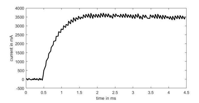
This mathematical description of the motor has to be verified to be useful for controlling the robot. This can be done by applying the same input to both the mathematical model as well as the physical motor and comparing the results afterwards. We have applied specific values between 1V and 12V on both systems. The measurement of the current through the motor after increasing the voltage from 0V to 6V can be seen in figure 1 as known from PT1-systems. In our system the measured behavior of the real system fits very well on the mathematical model using values from the datasheet with only smaller modifications to the parameters in order to decrease modeling errors.

To increase the precision of the mathematical model we added a dead time of 1 clock cycle, so the system results in

$$x_{k+1} = \begin{bmatrix} A_d & 0 \ 1 & 0 \end{bmatrix} x_k + \begin{bmatrix} B_d \ 0 \end{bmatrix} u_k = A_d^+ x_k + B_d^+ u_k$$

$$y_k = \begin{bmatrix} 0 & C_d \end{bmatrix} x_k = C_d^+ x_k$$

2.2 State-Space Controller

In systems in which are states that can't be measured, an observer is necessary to estimate this states. In the given system the state for the dead time is not a measurable value, so an observer is needed.

The Observer

The observer gain is calculated by the Ackermann-Formula

$$l = \sum_{i=0}^{n} (a_{Bi} - a_i) A_d^{+i} t_B$$

as $t_B$ is the last column of the inverse matrix for observability

$$Q_B = \begin{bmatrix} C_d^+ \ C_d^+ A_d^+ \end{bmatrix}$$

$$Q_{B,inv} = Q_B^{-1}$$

The coefficients $a_0$ and $a_1$ are calculated by

$$\det(zI - A_d^+) = a_0 + a_1 z + z^2$$

The coefficients $a_{B0}$ and $a_{B1}$ are degrees of freedom that set the dynamic of the observer and are given by

$$(z - \lambda_1)(z - \lambda_2) = a_{B0} + a_{B1}z + z^2$$

while $\lambda_1$ and $\lambda_2$ are the discrete eigenvalues of the observer and have to be chosen between 0 and 1. An eigenvalue closer to 0 represents a faster convergation of the estimation, an eigenvalue closer to 1 the opposite.

The Controller

Further an error model for constant errors is used. This model is described by

$$x_{k+1} = x_k$$

which expands the state-space-model that now results in

$$x_{ext,k+1} = \begin{bmatrix} A_d & 0 & 0 \ 1 & 0 & 0 \ 0 & C_d & 1 \end{bmatrix} x_{ext,k} + \begin{bmatrix} B_d \ 0 \ 0 \end{bmatrix} u_k = A_{ext} x_{ext,k} + B_{ext} u_k$$

The controller can be calculated by the Ackermann-Formula

$$k^{T} = \sum_{i=0}^{n} (a_{Ri} - a_{i}) t_{R} A_{ext}^{i}$$

with $t_R$ as the last row of the inverse matrix of controllability

$$Q_s = \left[ B_{ext} \ A_{ext} B_{ext} \ A_{ext}^2 B_{ext} \right]$$

$$Q_{s,inv} = Q_s^{-1}$$

The coefficients $a_0$ to $a_2$ have to be calculated by

$$\det(zI - A_{ext}) = a_0 + a_1 z + a_2 z^2 + z^3$$

The coefficients $a_{R0}$ to $a_{R2}$ are degrees of freedom that set the dynamic of the controller and are achieved by

$$(z - \lambda_1)(z - \lambda_2)(z - \lambda_3) = a_{R0} + a_{R1}z + a_{R2}z_2 + z^3$$

while $\lambda_1$ to $\lambda_3$ are the discrete eigenvalues of the controller and have to be chosen between 0 and 1.

The Result

This results in the following formulas for the observer

$$\hat{e}x_{k+1} = (A_d^+ - lC_d^{+T})\hat{e}x_k + B_d^+ u_{R,k} + ley_k$$

with

$$ey_k = y_{desired,k} - y_{measured,k}$$

and the controller

$$u_{R,k} = [k_0 \ k_1 \ k_2] \ ex_{k,ext}$$

2.3 Dynamic Feedforward

The dynamic feedforward can be achieved by first calculating the discrete transfer function of the system by

$$G(z) = C_d^+ (zI - A_d^+)^{-1} B_d^+$$

The feedforward is calculated by

$$G_{AW}(z) = G_{WS}(z)G(z)^{-1}$$

while $G_{WS}(z)$ is a degree of freedom and sets the desired dynamic for the feed-forward.

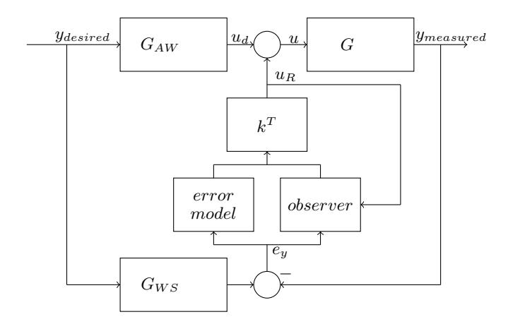
The resulting system is shown in figure 2.

2.4 Outlook

To further increase the performance of our robots, we plan to realize a discrete multi-variable state-space controller with a flat-based feedforward.

3 Strategy (A.I.)

In 2013, some serious design flaws led us to discontinue our Skills-Tactics-Playsbased strategy (it was not an exact implementation of the STP paper [1] but something similar). One of many problems was that we had to specify tasks for every robot in every possible situation. Instead of trying to work around these issues, we saw this as an opportunity to try out something new. In this chapter we will explain the structure of our current strategy (named Marvin) as well as our experiences, the positive and the negative ones. Keep in mind that the explanations are focused on the fundamentals of our strategy.

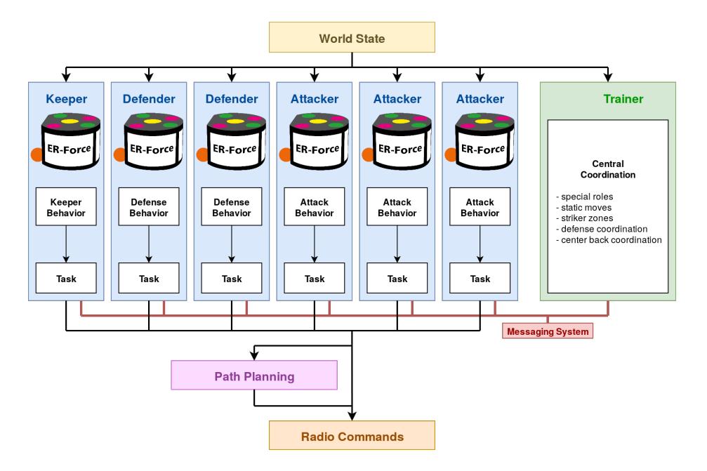
Figure 3 shows a high-level overview over the design of our strategy. The main difference between Marvin and a standard STP design is that our approach is headless to some extent, meaning that there is no instance that directly controls multiple robots at once. Instead, each robot is controlled by exactly one agent (drawn as a blue box).

In other words, each robot has its own mind.

3.1 Agents

Agents are the core element of Marvin's design. Each agent can perceive the world (ball, robots, referee commands, etc.), modify the world by sending instructions to its robot and communicate with other agents via a messaging system. This means that an agent has to make high-level decisions based on the world state as well as generate low-level commands to send to the robot. To subdivide this enormous job, the decision making is split into multiple layers:

• There are different agent types: attackers, defenders and keepers. The number of attackers and defenders can be changed dynamically. The deciding factor is the referee command. When the opponent performs a freekick or the Stop command is given, we have less attackers. Likewise, if we perform a freekick, we increase the number of attackers. Whenever an agent changes its type it has to be recreated.
• Depending on the type, each agent has a list of behaviors it can perform. Attackers for example can execute a freekick, duel an opponent or assist an attack. Defenders can mark an opponent, stay in proximity of the defense area or clear the ball, amongst other behaviors of course. In order to choose a behavior, the list of possible behaviors is traversed. The first behavior that fits the current state will be selected. If this behavior is different from the choice of the last iteration, the newly selected behavior will be restarted. If it is the same as in the last iteration instead, it will just continue to run.
• A behavior decides, what to do, mainly by choosing a task. A defender that runs the man-mark behavior can follow the opponent around the map or throw its plastic-coated body in the line of a goal shot to deflect the ball at the last possible moment. Likewise, an attacker that performs a freekick can either pass or shoot towards the goal.
• A task on the other side specifies, how to do it. Take the ShootGoal task as an example. This task searches for a position to shoot at and decides whether to shoot linearly or chip. The tasks are comparable to the tactics of a STP design. Unlike behaviors, tasks are usable by agents of different types. For example, a defender that happened to get the ball may pass it to a teammate, which is usually a task that attackers do.

3.2 Messaging System

To prevent utter chaos, the agent's decisions have to be communicated. In Marvin, we implemented a messaging system to fulfill this task. Each agent has an outbox which collects all outgoing messages as well as an inbox. Between two iterations of the strategy, all messages will be delivered. As a consequence, all messages have a delay of one iteration.

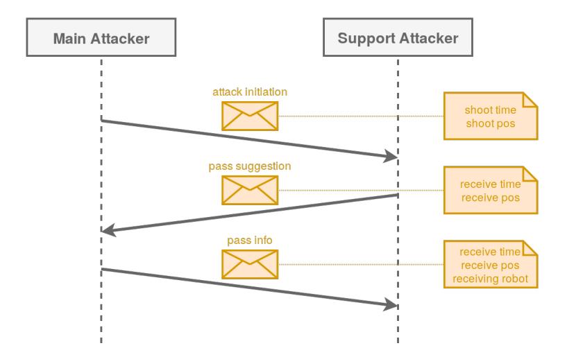
Figure 4 shows an exemplary usage of messages in Marvin. In this scenario, there are two attackers: the main attacker and a support attacker. The main attacker is the agent whose robot will try to get the ball (either by receiving a previous pass or by picking up a stray ball). Even though it is not in possession of the ball yet, the main attacker already looks for possible attack maneuvers.

• Every iteration the main attacker estimates when and from which position it will be able to shoot the ball and broadcasts it to all other robots using the attack initiation message.
• Each support attacker proposes a pass destination (time and position) to the main attacker using the pass suggestion message.
• The main attacker selects the best one and (if it decides to pass the ball at all) communicates its decision to all agents via the pass info message. The time and pos may differ a bit from the original suggestion. The main attacker guarantees that the ball will be at the position at the time announced in the pass info message. The support attacker is free to do whatever it wants in the meantime, like sidestep to distract the opponent defenders.

As soon as the main attacker has shot the ball towards the support attacker, the roles are swapped and the pass receiver is in charge of looking for another target to shoot at.

3.3 Trainer

Role Assignment In the above-mentioned case it is quite clear which robot will be the main attacker. However, in most cases, it is far from obvious for a single agent to decide whether it should try to get the ball or not. It would be helpful to have one module that decides which robot is the main attacker. This is the job of the trainer in Marvin. Like agents, the trainer is also connected to the messaging system. To select a main attacker, every attacker (and in some cases defenders) sends a message to the trainer containing an estimation of how well the robot fits the given role. The trainer will then pick the best one and broadcast this decision to every agent.

Groups Probably the most important feature of the trainer is the ability to coordinate groups. There are a couple of groups in Marvin, solving all kinds of challenges, from high-level task assignments to position calculations. Groups function as follows:

• Every agent that wants to be part of a group sends an application message containing the group name to the trainer.
• The trainer executes the group handler for every group that has at least one member.
• The group handler sends out messages to all participants containing the results of the calculations.

Marvin uses groups to solve the following problems:

• The logic of Marvin's defense coordination is pretty much all concentrated in the trainer. Every defender applies for this group. The trainer then evaluates the dangerousness of the opponent robots and assigns defenders accordingly. These defender assignments are sent to the respective agents via the messaging system. A detailed description of Marvin's defense can be found in last year's ETDP [2].
• Like the strategy of most other teams, Marvin has some form of defenders that move along the defense area, called center backs. To ensure fluid movement without collisions, the positioning of the center backs is calculated centrally.
• To spread the strikers, we assign a zone to each attacker (support attacker as well as main attacker), similar to the approach described by CMDragons [3].
• A fairly new feature of Marvin is the option to define static moves. Static moves are preplanned attack combinations of multiple robots, comparable to plays in the STP design. Every attacker applies for this group. Once a appropriate move is found, the move chooses tasks or even behaviors for every participating robot. These choices are sent to the agents via messages.

3.4 Evaluation

The change from 5v5 to 6v6 a couple of years ago was something we struggled with a lot. Our former strategy always used a hard coded number of attackers. With the addition of another robot, we had to rewrite most of the attack plays. This is why we wanted to create a strategy that works independently of the number of robots. In Marvin, depending on the referee command, a percentage of our robots are attackers and all remaining robots will be defenders, except the keeper of course. This lets us play 4v4 show matches in our lab, 6v6 tournament matches as well as 8v8 matches next year. The ability to just put some robots on the field and let the strategy run without having to change anything is a feature that already proved to be handy in a lot of cases.

The most significant advantage of an agent-based approach like Marvin is that implementing a dynamic attack is fairly easy. Figure 4 shows how the agents have to communicate to plan a pass in the run. At the RoboCup 2017 we mainly used the dynamic attack, with great success. It sometimes even outperformed the static moves in standard situations. Maybe it's because we are quite inexperienced in designing static moves (we only had two moves at that time), but nevertheless, being able to initiate multi-pass attacks after intercepting opponent passes or after winning duels is worth a lot.

It all comes at a cost. It may not seem like a problem, but the one iteration delay of messages adds more complexity to the system than anything else. The difficulty is that at any given iteration, you don't only have the current calculations but also the results of the previous iterations that were sent via messages. Take the pass coordination as an example. When the main attacker receives the pass suggestion message, its content relies on attack initiation data from two iterations ago. The actual time difference is not the problem here (Marvin runs at 100 iterations per second), but having multiple sets of the same data can be confusing.

All in all, Marvin is quite a success. Sure, we've encountered a lot of issues on the way and developing Marvin would not have been without the use of sophisticated debugging techniques, which are described in the following section. However, using a agent-based approach was a great improvement and we will continue to develop Marvin in the coming years.

4 Debugging Techniques

As our software is increasing in complexity, it is getting ever harder to properly find and fix bugs that appear during tests or a game. Like many other teams we utilize a simulator to be able to test our software faster, and can record real games and simulated games to log files for further analysis. In these logs we capture the world state after our tracking algorithm as well as debug outputs. As we are currently not able to dump the whole strategy state in every frame, we explicitly write the debug information, which consists mainly of three types of output:

• pure text output
• visualizations that appear in an overlay over the field
• a hierarchical output in which we can write information for every robot regarding its current task and any information the task deems necessary for debugging

For some years, this was enough to properly develop our strategy. But this year, we introduced additional features that improved our debugging workflow.

Backlog As our log files grow to a rather large size (500 MB for a regular game), the creation of a log file during testing has to be explicitly enabled. But oftentimes during testing unexpected situations occur, in which case a log file would be valuable to have. Thus we introduced a feature that continuously holds the last 20 seconds of the game with all associated debug information in memory in a cyclic buffer. This backlog can then be saved into a regular log file in case it is necessary.

Strategy Replay Many bugs can be fixed with the visualizations that are present in a given log file. But unanticipated bugs often require further information about the exact state the strategy was in when triggering the bug. It is not feasible to create even more debug output since our framework already spends a significant amount of time for creating, saving and displaying debug information.

Thus we introduced a new mode to our log player, in which a modified version of the strategy is executed on the world states contained in the log file in order to reproduce the bug with additional debug information. It is important to note that the commands of the new running strategy regarding the robots are ignored in favor of continuing to replay the states contained in the log file. Multiple modifications to our system were necessary in order to properly reproduce issues. Two conditions must be met at all times for the replayed strategy state not to diverge from the original strategy state.

• The strategy must be given exactly the same world state as on the original execution. We previously only stored the inputs coming from the vision. However, as the extrapolation of our tracking code is dependent on the exact execution timing, the strategy would get slightly different world inputs than during the original run. This problem can be solved by saving the exact strategy input to the log file as well.
• The strategy must act fully deterministic. Multiple modifications where necessary to archive this goal:
  • Random number generation: Using random numbers can be beneficial in many situations. The pseudorandom number generator is seeded with the world time in every frame to guarantee that it will return the same results (given that it is called the same number of times) as in the recorded execution.
  • Lua tables: Our strategy is written in the LUA language whose main data structure are tables. These work similar to hashtables but can also behave like an array when using numerical indices. During iteration over all elements in a table the function pairs is used, which behaves like a hashtable iterator. However, the order of elements yielded by the iterator is not defined. In practice, LuaJIT will use the memory location of the contained elements to sort the hashmap. This means that since the allocator is not deterministic, multiple runs of LUA code containing a for loop iterating over a table will not iterate in the same order. All functions whose result depends on the iteration order of elements in a loop must thus be changed. Some functions generate a table themselves, in these places the output can be sorted to guarantee determinism. Some tables are too ingrained in the structure of our strategy to change them without a large amount of work, for example our messaging system (see 5.3). Here a feature of LUA 5.2 can be used where the pairs iterator can be customized by overwriting the pairs function for the table in question. This iterator can be crafted to sort the elements internally by a key that has to be chosen specifically for each kind of table. Note that this is only reasonable if the table only contains a small numbers of elements, otherwise a different method should be chosen.

Another option, which we didn't choose though, would be to patch Lua-JIT to keep track of the insertion order of elements into a table and using this as the key for sorting these tables. However, this incurs performance penalties as additional data must be kept track of.

The strategy replay is perfectly suited for debugging and creating analyzer functions which just compute a value based on the current game state. It is no longer necessary to recreate the specific game state a function should be tested on every time the code has changed. Rather one can just record the situation once and replay the strategy afterwards.

Note that it is not necessary for the log file to start at the point when the strategy was initially loaded. Although this would ensure that the replay is exactly the same as the original run, most replays will converge on the behavior seen in the log file. This is because our strategy does not have many internal states that are long lived and change the behavior drastically. A 20 second log file is sufficient for the replay to converge on the log files actions at the end of the log (where the issue usually occurs when a backlog is recorded).

5 Conclusion

In this ETDP, we described what we think are the most significant factors that lead to our success on the RoboCup 2017: the improvements in motion control, our strategy design and the debugging techniques that enabled us to develop the strategy in the first place. We all hope that the information is understandable and useful to you and we are looking forward to hearing your feedback.

References

1. Browning, B., Bruce, J., Bowling, M., Veloso, M.: STP: Skills, tactics and plays for multi-robot control in adversarial environments. Journal of Systems and Control Engineering 219(1) (2005) 33–52
2. Lobmeier, C., Blank, P., Bühlmeyer, J., Burk, D., Danzer, A., Kronberger, S., Niebisch, M., Eskofier, B.M.: ER-Force Extended Team Description Paper RoboCup 2017 (2017)
3. Mendoza, J.P., Biswas, J., Zhu, D., Wang, R., Cooksey, P., Klee, S., Veloso, M.: CMDragons 2016 Extended Team Description Paper (2016)