RoboDragons 2018 Extended Team Description
Masahide Ito, Hiroyuki Kusakabe, Yusuke Adachi, Reona Suzuki, Jiale Du, Yuta Ando, Yuto Izawa, Shogo Isokawa, Taiga Kato, Tadashi Naruse
School of Information Science and Technology, Aichi Prefectural University
Abstract RoboDragons is a team of Aichi Prefectural Univeristy in the RoboCup Soccer Small Size League. In this paper, we presents the technical overview of our robots and their main changes from 2017 to 2018. We introduced new robots—have been developed in 2016—to the last RoboCup, but found out some issues on the hardware through the games. As one of hardware improvement, we redesigned a part of the dribbler so as to receive a passed ball more unfailingly; in the software part, we considered a trajectory tracking controller based on the model predictive control approach.
1 Introduction
RoboDragons is a team of Aichi Prefectural University (APU), participating in the Small Size League (SSL) of RoboCup Soccer. This team originated from Owaribito—a joint team between APU and Chubu University—which was founded in 1997. In 2002, since two universities have been ready to manage each individual team, APU built a new team, RoboDraongs. After that, RoboDragons has been participating in the SSL, including activities as CMRoboDragons—a joint team with Carnegie Mellon University in 2004 and 2005. Our best record was the second place in 2009. We also finished twice in the third place (2007 and 2014) and four times in the fourth place (2004, 2005, 2013, and 2016). In RoboCup 2017, we placed fifth out of twenty teams.
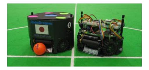
This paper summarizes the technical information of RoboDragons 2018, which includes the main changes from 2017 to 2018. We will use the seventh-generation (7G) robots (Fig. 1) in RoboCup 2018 as in last year. But, on the basis of the issues that we found out in RoboCup 2017, we have tried to improve the robots. As one of hardware improvement, we redesigned a part of the dribbler so as to receive a passed ball more unfailingly; in the software part, we considered a trajectory tracking controller based on the model predictive control approach.
2 Overview of RoboDragons System
2.1 Hardware Part
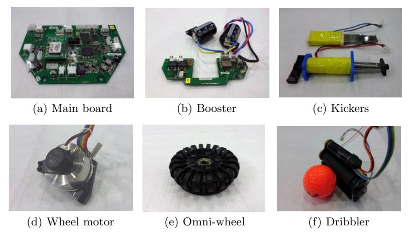
Figure 2 and Table 1 summarize the hardware configuration of the 7G robot. The 7G robots were developed in 2016. The most design is inherited from the 6G robot, but some components—such as the kickers and the dribbler—have been changed. See the details in our previous ETDP [1].
The last RoboCup was the first time that we used the 7G robots. They have carried the tough competition through to the end, but some technical issues on the hardware emerged in the latter schedule. One of them related to the dribbler.
We changed the alighment of the front wheels and rear wheels on the development of the 7G robots. Those wheels of the 7G robots are symmetrically aligned while the those wheels of the 6G robots were asymmetrically aligned. The reason was that the symmetric alignment would yield simplifying control of the robot motion. This change, however, gave not only such effect but also shortening the width of the dribbler. As a result, the robots often failed to receive a passed ball.
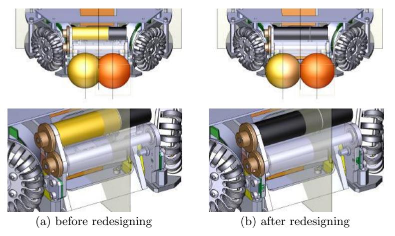
Redeveloping the dribbler costs high. So, we focused on side brackets of the dribbler. There were some spaces where we might whittle down, while there was ball detectors. Whittling down the spaces and redeveloping a new smaller ball detector achieved to make the place—where a ball can touch the dribbling roller—wider as shown in Fig. 3. In fact, the available width for a ball on the dribbling roller increases from 33.65 millimeters to 41.2 millimeters.
Description of main hardware components.
| Device | Description |
|---|---|
| Main board (Fig. 2 (a)) | CPU: SH2A (Renesas Electron. Corp.) operating at 197 MHz. FPGA: Spartan-6 (Xilinx) including peripheral circuits. |
| Booster (Fig. 2 (b)) | Capacitance of capacitor: 4400 µF. Conversion from 15.2 V DC to 150–200 V DC. Electric charge takes about 3 s for 200 V output. |
| Kickers (Fig. 2 (c)) | Material: 7075 alum. alloy. Solenoid: a coil wound by ϕ 0.6 mm enameled wire. Straight kicker can kick a ball at over 8 m/s; chip kicker can kick a ball as far as max. 3 m distance. |
| Omni-wheel (Figs. 2 (d) and (e)) | Four omni-wheels driven by Maxon "EC 45 flat 50W". Gear reduction ratio between motor and omni-wheel is 21:64. Each omni-wheel has 20 small tires in circumference. Diameter: omni-wheel 55 mm, small tire 12.4 mm. |
| Dribbler (Fig. 2 (f)) | One roller driven by Maxon "EC 16 30W". Roller: alum. shaft with non-repulsive rubber; 16 mm in diameter and 61 mm in length Radio system IEEE 802.11abgn 2.4/5 GHz wireless LAN. |
| Ball detector | Infra-red light emission diode and photo diode pair. Accelerometer BOSCH BMA250 (3-axis (range: ±2 G to ±16 G)) |
| Gyroscope | InvenSence ITG3400 (pitch, roll & yaw (range: ±250 deg/s)) |
2.2 Software Part
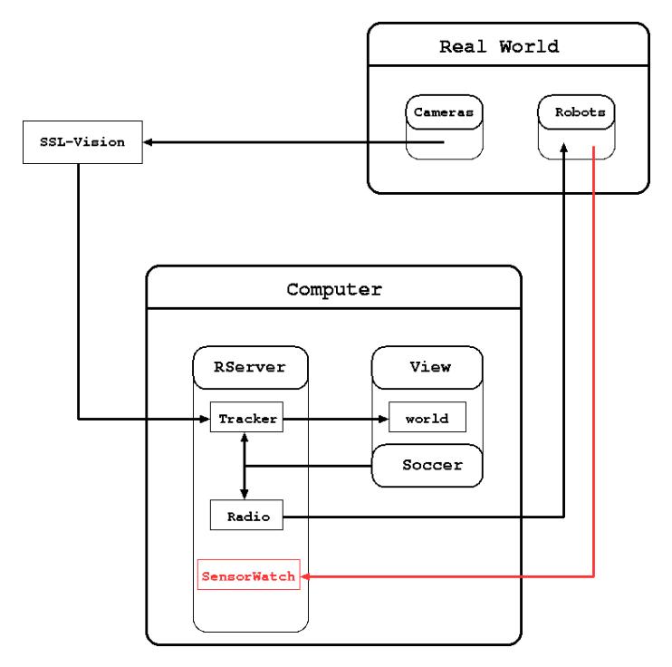
Figure 4 depicts an overview of our software system, which is mainly composed of three modules as follows:
The Rserver module receives the data from the SSL-Vision server, and then the Kalman filter in the Tracker submodule estimates the states of the ball and robots. The estimated states with the other information are shared among all modules. The Rserver sends a command packet to all robots through the Radio submodule; the SensorWatch submodule receives the information from the robots.
The View module provides a graphical user interface that a human operator can know the game situation and also can send the referee commands for tests.
The Soccer module chooses the best strategy for the current situation, assigns each robot a role based on the chosen strategy, and computes a motion command to perform the role for each robot.
See our ETDP 2017 [1] as for a bi-directional communication and the packets between the host computer and each robot.
As stated in Subsection 2.1, we redesigned the side brackets of the dribbler so as to receive a passed ball more unfailingly. For the same purpose, we also concentrated on improving the accuracy of robot motion. The detail is explained by next section.
3 Trajectory Tracking Controller based on Model Predictive Control
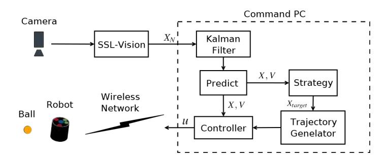
A robotic soccer team in the SSL generally adopt the same control system as depicted in Fig. 5. In this figure, a command PC has a (feedback) controller to track a desired/planned trajectory; each robot also utilizes a kind of feedback controller—like a PID controller—with Pulse Width Modulation to control DC brushless motors connected to omni-wheels. Let's focus on the control flow of the command PC, especially around a trajectory generator and a controller. The trajectory generator plans a trajectory based on the (sub-)target position given by a strategy; the controller compensates the error so that the actual state of a robot can track the planned trajectory.
In these years, RoboDragons have adopted online updated trajectory instead of a pair of the trajectory generator and controller. It is similar to what Skuba have presented in their ETDP 2011 [2]. This approach is simple and effective, but does not work well sometimes because the rapid growth of the SSL has required the high accuracy for some plays. We need control approaches so as to elicit performance of the hardware maximally and safely.
Model Predictive Control (MPC) [3] has recently attracted the attention of engineers and researchers. It is a kind of online optimization method including future prediction, and also can deal with the constraints. This approach has been already applied into RoboCup Soccer SSL [4], Middle Size League [5], and their similar setting [6].
This section gives a trajectory tracking controller based on the linear MPC approach. The proposed MPC controller handles velocity constraints in a different way with the conventional controllers [4, 6]. The performance of the proposed controller is evaluated by experimental results.
3.1 A Kinematic Robot Model
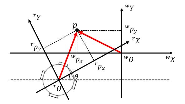
Assume that all frames in this paper are planar and right-handed systems. Locate the world frame $\Sigma_w$: $^w O^w X\ ^w Y$ at the center of the soccer field, where its $^w X$-axis heads to the opponent's goal. Also, locate the robot frame $\Sigma_r$: $^r O^r X\ ^r Y$ at the center of the robot, where its $^r X$-axis heads to the robot's front. The relationship between the two frames is depicted in Fig. 6. We specify the reference frame of variables and vectors by using the left superscript, e.g., $^w \boldsymbol{p} = [\ ^w p_x,\ ^w p_y\ ]^T$.
Suppose that the robot motion can be represented as a linear time-invariant continuous-time system. Then, by focusing on only translational motion of the robot for simplicity, we get the following state space model:
$$\frac{\mathrm{d}}{\mathrm{d}t}\boldsymbol{x}(t) = \begin{bmatrix} \alpha_x & 0\ 0 & \alpha_y \end{bmatrix} \boldsymbol{u}(t - H_w T_s),\tag{1a}$$
$$\mathbf{y}(t) = \mathbf{x}(t),\tag{1b}$$
where $\boldsymbol{x} := [\ ^r r_x, ^r r_y\ ]^T$, $\boldsymbol{u} := [\ ^r v_x, ^r v_y\ ]^T$, $\alpha_x$ and $\alpha_y$ are scaling parameters for the associated velocities, $T_s$ is sampling period, and $H_u T_s$ represents the deadtime on communication from the command PC to each robot, respectively. An MPC controller generally utilizes the discrete-time model of (1). Discretizing (1) gives
$$\boldsymbol{x}(k+1) = \begin{bmatrix} 1 & 0 \ 0 & 1 \end{bmatrix} \boldsymbol{x}(k) + \begin{bmatrix} \alpha_x T_s & 0 \ 0 & \alpha_y T_s \end{bmatrix} \boldsymbol{u}(k - H_w), \tag{2a}$$
$$\mathbf{y}(k) = \mathbf{x}(k). \tag{2b}$$
Due to the hardware limitation, the control input is subject to the following constraint:
$$|\boldsymbol{u}| \le \bar{v},\tag{3}$$
where $\bar{v} \in \mathbb{R}^+$ is the maximum speed of the translational velocity.
3.2 Model Predictive Tracking Controller with Transformed Velocity Constraints
In the linear MPC framework, we must represent a control objective as a performance index (or an objective function) of the quadratic form with linear constraints. Our control objective is trajectory tracking. To achieve it, the following performance index can be straightforward considered:
$$V(k) = \sum_{i=H_w}^{H_p} |\hat{\boldsymbol{y}}(k+i|k) - \boldsymbol{y}{\text{ref}}(k+i|k)|{\boldsymbol{\mathcal{Q}}(i)}^2 + \sum_{i=0}^{H_u-1} |\hat{\boldsymbol{u}}(k+i|k) - \boldsymbol{u}{\text{ref}}(k+i|k)|{\boldsymbol{\mathcal{R}}(i)}^2, \quad (4)$$
where $\hat{\boldsymbol{u}}$ and $\hat{\boldsymbol{y}}$ are controlled input and output for prediction in the MPC controller, $\boldsymbol{y}{\text{ref}}$ and $\boldsymbol{u}{\text{ref}}$ are set-point trajectories (like reference trajectories) for $\hat{\boldsymbol{u}}$ and $\hat{\boldsymbol{y}}$, $H_p$ and $H_u$ are prediction horizon for $\hat{\boldsymbol{u}}$ and $\hat{\boldsymbol{y}}$, and $\boldsymbol{\mathcal{Q}}$ and $\boldsymbol{\mathcal{R}}$ are weighting matrices, respectively.
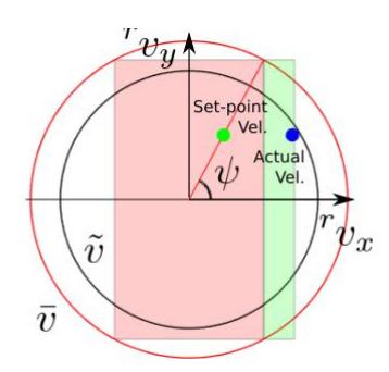
The most problem in this design is how we should deal with the velocity constraint (3) which is NOT linear. For this problem, we propose a solution by using transformation based on the set-point trajectory for the controlled input. On the $^r v_x$–$^r v_y$ plane as shown in Fig. 7, let the angle between $\boldsymbol{u}_{\text{ref}}$ and $^r v_x$ as $\psi$. By using $\psi$, we can decompose $\bar{v}$ into $\bar{v}_x$ and $\bar{v}_y$ as follows:
$$\bar{v}_x = |\bar{v}\cos\psi|,\tag{5a}$$
$$\bar{v}_y = |\bar{v}\sin\psi|. \tag{5b}$$
The decomposed limits transform the constraints (3) into
$$|^r v_x| \leq \bar{v}_x \quad \text{and} \quad |^r v_y| \leq \bar{v}_y.$$ (6)
If you pay attention to the case that the actual velocity accidentally goes out of the constraints, we can use the following equations instead of (4) and (5):
$$V(k) = \sum_{i=H_w}^{H_p} |\hat{\boldsymbol{y}}(k+i|k) - \boldsymbol{y}{\text{ref}}(k+i|k)|{\boldsymbol{Q}(i)}^2 + \sum_{i=0}^{H_u-1} |\hat{\boldsymbol{u}}(k+i|k) - \boldsymbol{u}{\text{ref}}(k+i|k)|{\boldsymbol{\mathcal{R}}(i)}^2 + W \sum_{i=0}^{2(H_u-1)} \epsilon_i, \quad (7)$$
$$\bar{v}_x = |\bar{v}\cos\psi| + \epsilon_x,\tag{8a}$$
$$\bar{v}_y = |\bar{v}\sin\psi| + \epsilon_y,$$ (8b)
where W is a weighting parameter and $\epsilon_i$ is called a slack variable. The slack variables contribute relaxing the constraints if any. See Fig. 7 to find out the light green area expanded by the slack variables.
Finally, in order to obtain actual control input, we need to solve a Quadratic Programming (QP) problem, i.e., to minimize the performance index (4) or (7) under the velocity constraints (6) with (5) or (8). For this, we can use CVX-GEN [8] and YALMIP [7], etc.
3.3 Experimental Validation
We evaluated the performance of the proposed MPC controller by the following experiment:
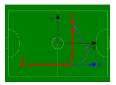
- The robot rests at Point S and waits for starting.
- The robot drives to Point P as the initial target position.
- The target position changes to Point G at the moment when the robot reaches within 2 meters of Point P.
- The robot goes to Point G while turning left.
- The experiment ends, when the robot arrives at Point G.
For comparison,
- the online updated trajectory as in [2]; and
- the following feedback controller based on pole placement for error system between the actual response and set-point trajectory:
$$\boldsymbol{u}(t) = \boldsymbol{u}_{\text{ref}}(t) + \boldsymbol{K}p { \boldsymbol{y}{\text{ref}}(t) - \boldsymbol{y}(t) }$$ (9)
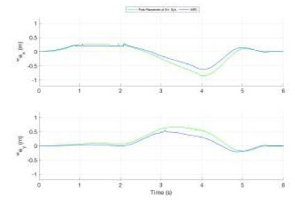
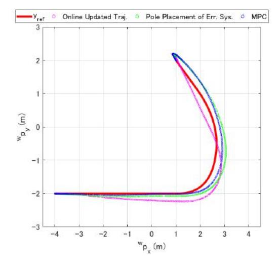
were also tested by same experiments. Figure 9 shows the experimental results with the following parameters: $\alpha_x = 0.9924$, $\alpha_y = 0.9777$, $H_p = H_u = 10$ steps, $H_w = 1$ step, $\boldsymbol{Q} = 255 \boldsymbol{I}_2$, $\boldsymbol{R} = 15 \boldsymbol{I}_2$, $W = 400$, and $\boldsymbol{K}_p = \boldsymbol{I}_2$, respectively.
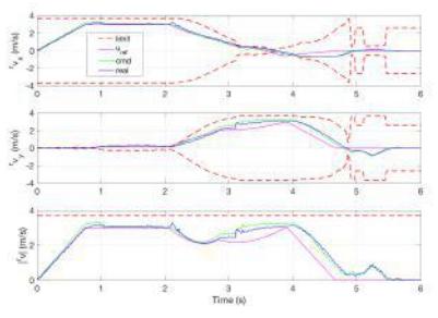
From Fig. 9 (a), command/actual velocities (green and blue) were mostly between the upper and lower limits; some parts of them went over the limits because of the slack variables. In Figs. 9 (b) and (c), it is hard to find the performance differences among three kinds of methods. However, Table 2 summarize the results with respect to tracking error and arrival time, which indicates that the proposed MPC controller is slightly better than the other methods.
Tracking Error and Arrival Time
| (Max.) | Tracking Err. (Ave.) | Arrival Time | |
|---|---|---|---|
| Online updated traj. as in [2] | 1.076 m | 0.350 m | 389 frame |
| Pole placement of Err. Syst. | 1.028 m | 0.224 m | 396 frame |
| Proposed MPC | 0.695 m | 0.203 m | 367 frame |
4 Concluding Remarks
We have presented the system configuration of RoboDragons 2018 robots. The main novelties of this ETDP are to improve the side brackets of the dribbler and also to introduce a new trajectory tracking controller based on model predictive control. Our robots will succeed to pass the ball between teammates more frequently than last year.
Acknowledgement
This work was supported by Aichi Prefectural University and JSPS KAKENHI Grant Number JP16K00430.
References
- Adachi, Y., Kusakabe, H., Suzuki, R., Du, J., Ito, M., and Naruse, T.: "RoboDragons 2017 Extended Team Description," RoboCup Soccer Small Size League, 2017.
- Chaiso, K. and Sukvichai, K.: "Skuba 2011 Extended Team Description," RoboCup Soccer Small Size League, 2011.
- Maciejowski, J.M.: "Predictive Control with Constraints," Prentice Hall, 2000.
- Zeng, Z., Lu, H., Zheng, Z.: "High-speed trajectory tracking based on model predictive control for omni-directional mobile robots," in Proc. the 25th Chinese Control and Decision Conference (CCDC'13), pp. 3179–3184, Nanjing, China, 2014.
- Zarghami, M., Fakharian, A., Poudeh, A.G., and Adhami-Mirhosseini, A.: "Fast and precise positioning of wheeled omni-directional robot with input delay using modelbased predictive control," in Proc. the 33rd Chinese Control Conference (CCC'14), pp. 7800–7804, Nanjing, China, 2014.
- Barreto S., J.C.L., Conceicao, A.G.S., Dorea, C.E.T., Martinez, L., and de Pieri, E.R.: "Design and implementation of model-predictive control with frictional conmpensation on an omnidirectional mobile robot," IEEE/ASME Trans. Mechatronics, Vol. 19, No. 2, pp. 467–7804, Nanjing, China, 2014.
- Löfberg, J.: "YALMIP: A Toolbox for Modeling and Optimization in MATLAB," in Proc. the CACSD Conference, Taipei, Taiwan, 2004.
- Mattingley, J. and Boyd, S.: "CVXGEN: A code generator for embedded convex optimization," Optimization and Engineering, Vol. 13, No. 1, pp. 1-27, 2012.