RoboJackets 2018 Team Description Paper

J. Almagro, J. Feltracco, R. Medrano, S. Naeem, J. Neiger, R. Osawa, E. Peterson, A. Shaw, M. Woodward

Georgia Institute of Technology

Abstract The RoboJackets RoboCup SSL team was founded in 2007 and has competed every year since. The team's objective this year was to improve the mechanical and electrical robustness of the overall system based on lessons learned from competition and continuous testing. In parallel, the team added more planning capabilities to the team's software and added firmware features. This paper describes these fleet upgrades and the progress made on their implementation.

1 Mechanical

The mechanical design for the fleet this year focuses on improving wheel traction and kicker reliability.

1.1 Drivetrain

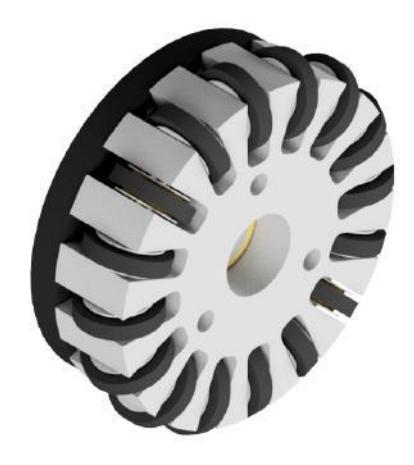
The assembly of the omniwheel remained the same as last year [1]. The body layer of the wheel was re-manufactured using wire electrical discharge machining. This method resulted in more precise dimensions of this component, which was desired due to the required connection between the wheel layer and the precisely machined inner gear. A major concern from last year's fleet was poor traction between the robots' wheels and the field. This was improved by adding rubber O-rings onto the metal rollers of the omniwheel shown in Figure 1. The change in tractive effort required to move the robot was determined by measuring the applied motor voltage when the robot's wheels began to slip, and comparing that voltage to that measured voltage for a robot with the metal rollers. This measurement resulted in an increased voltage from 1.6 volts to 2.7 volts, representing approximately a 60% increase in traction. A consequence of this roller change was a reduction in the number of rollers from twenty to sixteen.

1.2 Kicker

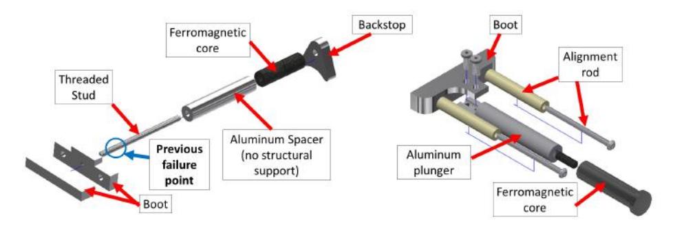
Previously, the kicker was assembled by connecting the boot to the steel core with a threaded stud and an aluminum spacer in between. The lack of structural support from the spacer resulted in the threaded stud snapping axially after repeated kicks. To resolve this problem, the kicker was redesigned such that the connection between the boot and the steel core was a solid aluminum rod. The boot is bolted on the rod and the steel core is connected with a threaded stud. This design change resulted in a better transmission of force from repeated kicks due to the larger cross-sectional area of the transmitting body. The exploded kicker assemblies are shown in Figure 2.

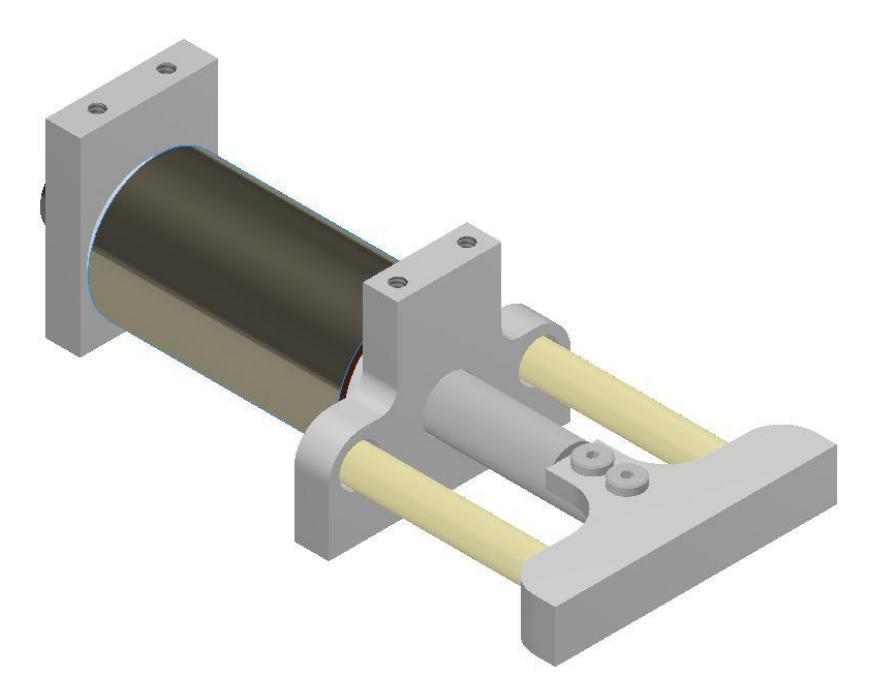
In addition, the kicker boot would rotate about the axis of the shaft, resulting in inconsistent kicks. This problem was addressed by adding alignment rods to the boot that go through the kicker solenoid stand, thus preventing rotation shown in Figure 3. Finally, the kicker spring would deform from repeated kicks, resulting in inaccurate kick speeds due to the spring not returning the kicker to a consistent position. This problem was addressed by using a spring with an increased number of windings and a higher spring constant changing from 1.61 lb/in to 2.181 lb/in.

2 Electrical

The electrical boards are heavily based off the last major redesign in 2015 [2] with a number of improvements and layout changes.

2.1 Control Board

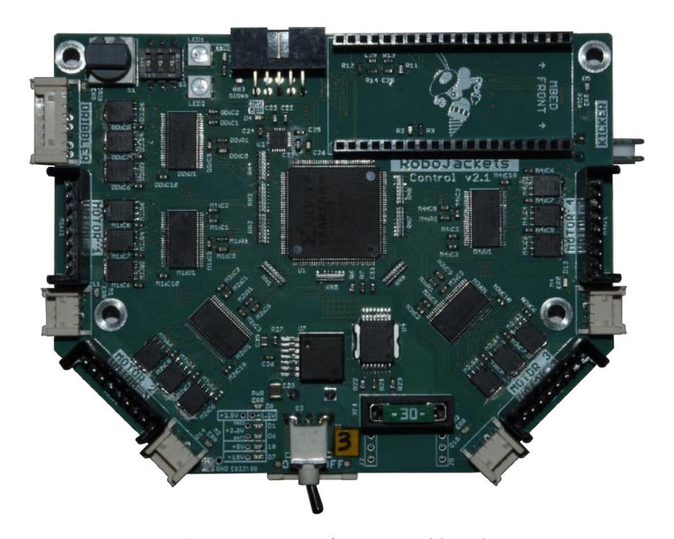
The control board and motor board have been merged into a single board. Originally, the control and motor boards were separated to allow for modularity, but the design caused more problems than it solved. Having separate boards decreased space efficiency, increased the cost of reordering boards, and caused many issues with the connectors (and subsequently, communication) between the boards. By combining the boards, space was saved, cost was reduced, and one of the main points of failure was removed.

The motor connectors have also been changed to be more intuitive to use and to require motor power and hall sensors to be connected at the same time, since one should not be connected without the other. The radio positioning was changed to a vertical position to reduce interference from the board and allow for the highest strength signal plane to face the base station. The fuse was changed to be a low profile while still easily removable. Larger capacitors have been added on the bottom of the board in order for the motor phases to reduce strain on motors when there is a large current draw.

2.2 Kicker Board

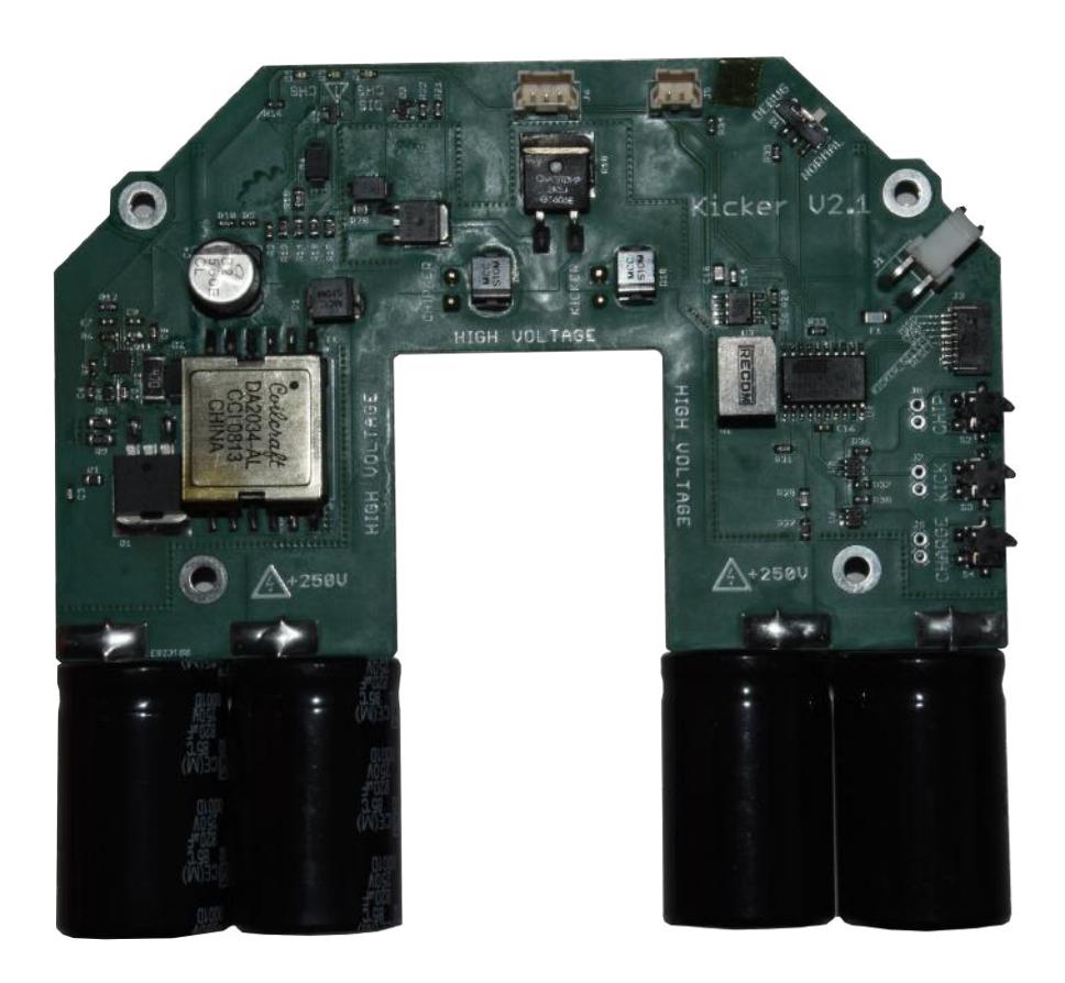
The new generation kicker board features an AVR microcontroller to allow complete standalone operation of the kicker board. The on-board peripherals include three user-programmable buttons, a slide switch to select normal operation or debug mode, and the breakbeam emitter and detector connections. The charge controller maintains the same chipset as the previous generation. LED indicators have also been added to report the auto-discharge status and the charge enable status. The IGBTs used in the previous generation to control the solenoid current have been replaced with power FETs. The IGBTs used in the past were overkill for the amount of current passed through the current solenoid. This switch helped improve energy efficiency for the discharge and allows for a lower profile. The routing of the board was also optimized to minimize the current noise induced on the SPI lines. The on-board microcontroller can be reprogrammed via the same SPI lines used for communicating kicker status with the primary microcontroller on the control board.

3 Software

(empty)

3.1 Over-The-Air Firmware Updates

Previously, in order to update any firmware each robot had to be pulled off the field and physically connected to a computer. This can be time consuming when testing firmware and frequently needing to update the robot firmware. Over-the-air firmware updates allow the robots to be reprogrammed over the existing radio connection on each of the robots. This functionality is part of a greater radio protocol restructure to allow additional types of radio packets. The MBED microcontroller updates its firmware by reading a binary file stored on its local file system so to update over radio a reliable file transfer protocol was implemented. This transfers the binary file from the computer to the MBED local file system and resets the MBED to read the new file. This can also be used to update the other firmware files stored on the local file system such as the kicker firmware, FPGA firmware, or any future configuration files.

3.2 Firmware Parameter Control

A remote parameter setting and debug variable reading system was set up to allow flexible writing and reading configuration and debug variables over radio communication. This allows for things such as quick tuning of the firmware PID. The debug variable reading was developed as a minor extension of the current radio protocol. The general structure is a control packet that is sent out from the base station, and then each robot responds after a delay in a reserved timeslot. Optional parameters were added to the command packet to request debug variables. Each robot then appends those variable values at the end of their response packets. The configuration variables were implemented with a new base station configuration packet. It can indicate that it applies to one or all the robots and specifies the variables and values it wants to set. The variables are identified using 8-bit identifiers. These variable enum lists are compiled into the base station and robot firmwares. The debug variables are also integrated into the logging and graphing system allowing easy visualization. This is especially useful for graphing velocity and acceleration for tuning PID configuration values.

3.3 Gyro Based Controller

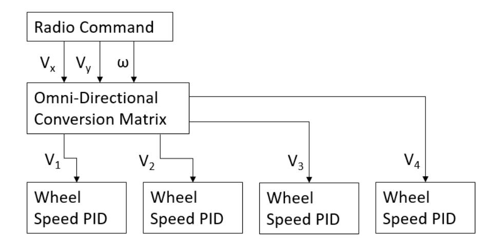
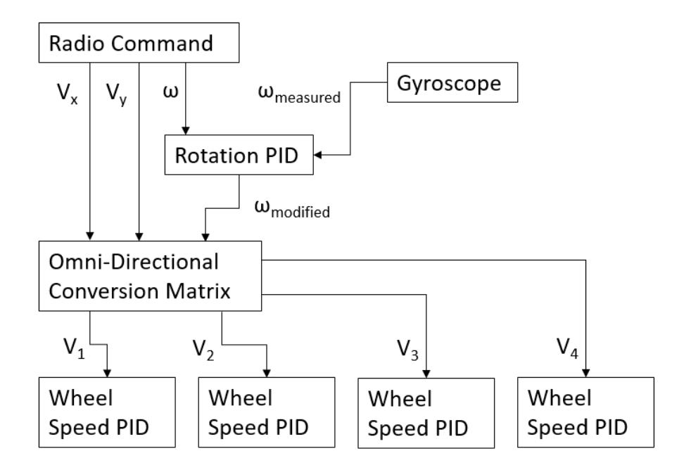
On a field with reduced traction, or at high robot speeds, the control system would tend to develop angular oscillations due to non-linear wheel slippage effects. In an effort to improve angular rate control, an on-board IMU (MPU-6050) was leveraged to sense an angular velocity of the robot. This measurement is used in a new outer control loop to drive the angular rotation setpoint of the previously designed control system. Before, a simple mapping was done from robot body velocities to wheel speeds as shown in [3], however now the rotational velocity setpoint is set to the output of a new controller that leverages the IMU's gyroscope reading along with the commanded rotational velocity. Thus, the new target angular robot velocity will attempt to counter disturbances in the angular rotation velocity of the robot. This system, therefore, counters wheel slippage effects that invalidate the mapping from robot body speeds to wheel speeds, at a lower layer of the control system, rather than relying on vision measurements to eventually propagate back to the control system.

3.4 Mirroring Real Life Defense

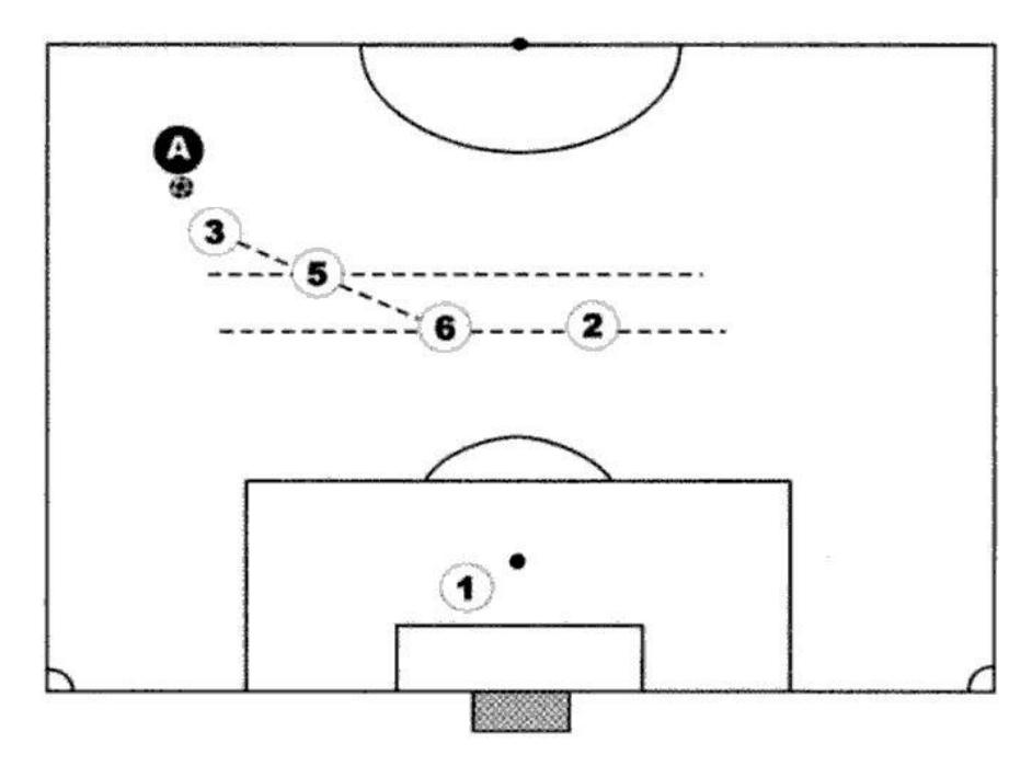
High level defensive techniques used in real life soccer were incorporated into the team's defense. In real life soccer, there are two basic objectives that need to be balanced [4]. The first is slowing down opponents play. This allows more time for the entire defense to move into position as well as eliminate many of the quick passing plays that are extremely difficult to defend against. The second objective is pushing opponents into making suboptimal decisions that are difficult to execute successfully.

Slowing down the offensive push can be done through overall positioning. In a real life 4-man defense, there is a diagonal that sweeps across the field shown in Figure 8. The specific positioning of the robots block the dangerous through passes while still leaving the defending robots in a position to react to other actions. Pushing opponents into suboptimal decisions can be done through marking the offensive players on an inside angle as shown by player 3 marking striker A in Figure 8.

3.5 Modeling the Success Chance of Passes and Shots

There are many uncertainties in RoboCup due to the fast nature of the game. It is essential that the metrics used to compare different high level plays account for these uncertainties. This is especially important for the more critical metrics, such as shot and pass chance of success.

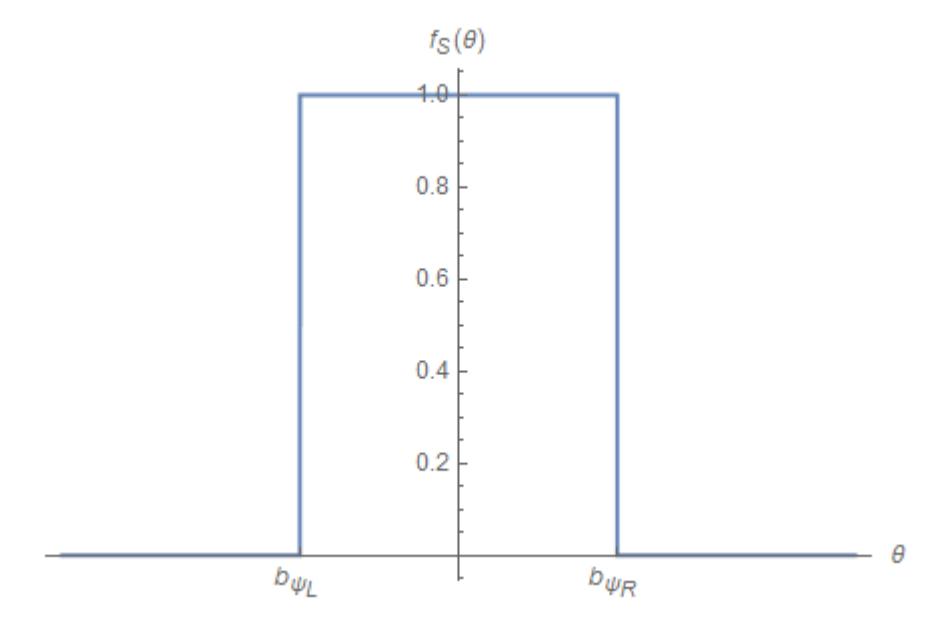
Consider the case where a robot is shooting on goal with no opponent robots on the field. Additionally, assume the kicker is extremely accurate with no variation in the kicking direction. The chance of success as a function of kick angle will just be a boxcar function with the edges at the goal posts, as shown in Figure 9, where θ is the angle of the kick from the kicker position, ψ$^L$ is the angle of the left goalpost from the kicker, and ψ$^R$ is the angle of the right goalpost from the kicker.

$$f_s(\theta) = b_{\psi_L, \psi_R}(\theta) \tag{1}$$

Let f$^r$$^n$ (x, y) be the probability that robot n will be at the position (x, y) ∆t in the future. Given the width of the robot w${robot}$ and a ball width w${ball}$, the length of the blocking segment w$^b$ can be calculated.

$$w_b = w_{robot} + w_{ball} \tag{2}$$

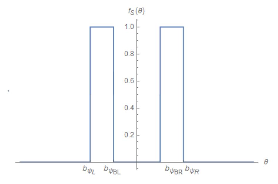
The blocking segment is perpendicular to the kicker-robot vector. Thus, the angle range blocked by the kicker is between ψ${BL}$ and ψ${BR}$, where d$_{kr}$ is the distance from the kicker to the opponent robot and φ$^r$ is the angle from the kicker to the robot. Therefore, f$_S$(θ) can be calculated for a single robot given the robots position on the field as shown in Figure 10.

$$\psi_B = \tan^{-1} \left( \frac{1}{2} \frac{w_b}{d_{kr}} \right) \tag{3}$$

$$\psi_{BL} = \phi_r - \psi_B \tag{4}$$

$$\psi_{BR} = \phi_r + \psi_B \tag{5}$$

$$f_s(\theta) = b_{\psi_L, \psi_R}(\theta) (1 - b_{\psi_{BL}, \psi_{BR}}(\theta)) \tag{6}$$

Equation 6 is the result given a specific robot location. If this location is expanded to be its own random distribution across the XY plane, the chance that a robot will block the ball becomes an integral over that area. This is specifically described as all locations which within w$^b$ 2 of the ball path vector at the kick direction θ as shown in Equation 7.

$$f_s(\theta) = b_{\psi_L, \psi_R}(\theta) \left(1 - \iint_{(x,y) \in d((x,y), \overrightarrow{K}) < \frac{w_b}{2}} f_{r_n}(x,y) \right) \tag{7}$$

Let B$^n$ be the event that an opponent robot n is in the area described by (x, y) ∈ d((x, y), −→K) $^$<W$^b$ 2 . Thus, Equation 7 can be rewritten as Equation 8 for the single robot case and Equation 9 for the multi-robot case.

$$f_s(\theta) = b_{\psi_L, \psi_R}(\theta) \left( 1 - P(B_n | \theta) \right) \tag{8}$$

$$f_s(\theta) = b_{\psi_L, \psi_R}(\theta) \left( 1 - (P(B_1 | \theta) \cup P(B_2 | \theta) \cup \dots \cup P(B_n | \theta)) \right) \tag{9}$$

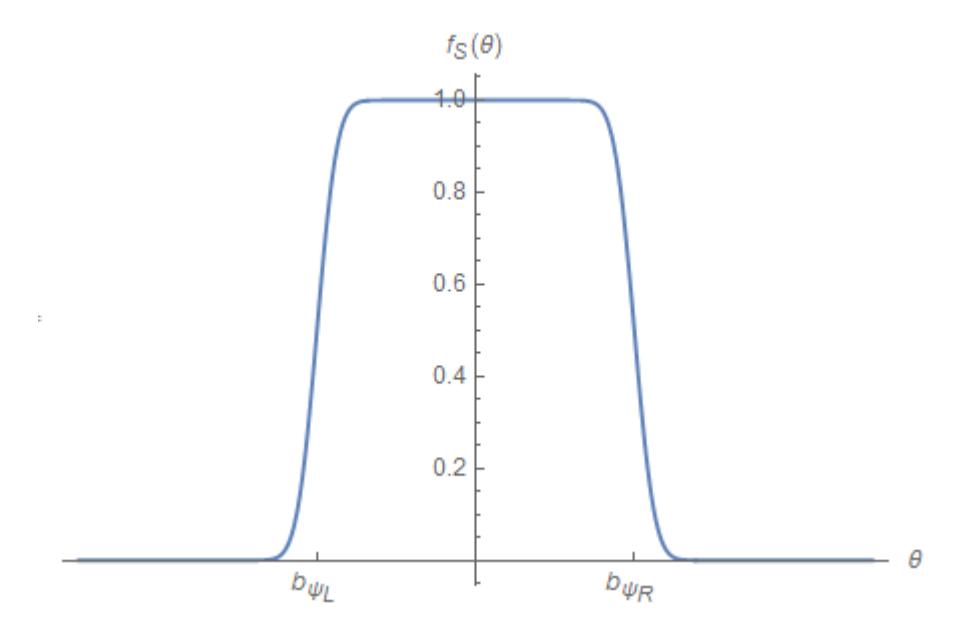
Revisiting the assumption made earlier about the kicking accuracy. Let f$_K$(ψ) represents a kicking distribution, where φ = 0 is the kick directly at the target location. In the simple case of no robots in Equation 1, it follows that the convolution of Equation 1 with the kicking distribution results in the overall chance of success at each kick angle θ shown in Equation 10 and in Figure 11.

$$f_s(\theta) = (f_K * b_{\psi_L, \psi_R})(\theta) \tag{10}$$

If the convolution is applied to the final multi-robot distribution in Equation 9, then it follows that the true shot success chance is 11.

$$f_s(\theta) = \left( f_K * \left( b_{\psi_L, \psi_R} \left( 1 - \left( P(B_1 | \theta) \cup P(B_2 | \theta) \cup \dots \cup P(B_n | \theta) \right) \right) \right) \right) (\theta) \quad (11)$$

One important assumption being made for f$_s$(θ) is that the path of the kicked ball is a straight line. The coordinate system transformations between the field locations and the angle of the kick will be significantly different if this was not the case.

3.6 Estimating the Model for Kick and Shot Chance

Due to the complexity in the model in both the integrals as well as the convolution, an estimation of the model must be made to allow for near real time evaluations during a game of soccer.

Computing $f_s(\theta)$ The predicted robot location $f_{r_n}(x,y)$ is estimated as a symmetric bi-variate normal distribution with the mean centered at the current robot location and a standard deviation $\sigma$ . This provides a few shortcuts when calculating the overall probability of a robot blocking the path of the ball when kicked.

Given that the ball only moves in a straight line, and the marginal distribution in any direction of a symmetric bi-variate normal distribution is a normal distribution, $P(B_n|\theta)$ is a scaled version of $\Phi(-\psi_B \leq \theta - \phi_r < \psi_B) + \epsilon(\theta)$ where $\epsilon(\theta)$ is the distortion from rectangular to polar coordinate system conversions. $\epsilon(\theta)$ is assumed to be zero. The scale of $P(B_n)$ is dependent on the difference between the distance between the target and the kicker, d, and the blocking robot and the kicker, $d_k r$ .

$$P(B_n|\theta) = \Phi\left(-\frac{\psi_B}{\sigma} \le \frac{\theta - \phi_r}{\sigma} < \frac{\psi_B}{\sigma}\right) \Phi\left(\frac{d_{kr} - d}{\sigma}\right) \tag{12}$$

Since the difference between $-\psi_B$ and $\psi_B$ is not dependent on $\theta$ , only on $d_k r$ , $\Phi\left(-\frac{\psi_B}{\sigma} \leq \frac{\theta - \phi_r}{\sigma} < \frac{\psi_B}{\sigma}\right)$ can be estimated by $\alpha\Phi\left(\frac{\theta}{\sigma l}\right)$ with a standard deviation of $\sigma l$ and a mean of 0. $\alpha$ represents the normalization coefficients for these distributions. As the standard deviations of the functions become smaller, it is possible for $\Phi\left(\frac{\theta}{\sigma l}\right)$ to become larger than one in some cases. It was found that normalizing $\Phi\left(\frac{\theta}{\sigma l}\right)$ to have a max of 1 resulted in the most accurate solution which results in an $\alpha=\frac{\sigma l}{\sqrt{2\pi}}$ . This substitution was primarily done to simplify the closed form solution when calculating the convolution.

For the multi-robot case, the union of the $P(B_n|\theta)$ for all n robots are simplified to just the addition of the individual probabilities. This results in sharper peaks when two blocking robots are near each other, but the error stays reasonably low. Additionally, instead of multiplying $b_{\psi_L,\psi_R}(\theta)$ with $\left(1-(P(B_1|\theta)\cup P(B_2|\theta)\cup ...\cup P(B_n|\theta))\right)$ , the two are added such that the final function to estimate the probability of success is Equation 13. The combination results in some underestimation of the true probability of success when evaluating near the boundaries of the target segment. When the convolution is fully evaluated, the resulting function is Equation 14. For the estimation, assume $f_k$ is a normal distribution with mean $\mu_k$ and standard deviation $\sigma_k$ .

$$f_s(\theta) = \left( f_K * (b_{\psi_L, \psi_R} - P(B_1 | \theta) - P(B_2 | \theta) - \dots - P(B_n | \theta)) \right) (\theta) \tag{13}$$

$$f_s(\theta) = \frac{1}{\sigma_k \sqrt{2\pi}} \left( \sum_{i=1}^n \left[ -\frac{e^{-\frac{(\mu_k + \phi_{r_i} - \theta)^2}{2(\sigma_k^2 + \sigma_{r_i}^2)}} \sqrt{2\pi}}}{\sqrt{\frac{1}{\sigma_k^2} + \frac{1}{\sigma_{r_i}^2}}} \right] + \sqrt{\frac{\pi}{2}} \left( \frac{1}{\sqrt{\frac{1}{\sigma_k^2}}} - \sigma_k \operatorname{erf}\left[\frac{\psi_L + \mu_k - \theta}{\sqrt{2}\sigma_k}\right] \right) - \sqrt{\frac{\pi}{2}} \left( \frac{1}{\sqrt{\frac{1}{\sigma_k^2}}} - \sigma_k \operatorname{erf}\left[\frac{\psi_R + \mu_k - \theta}{\sqrt{2}\sigma_k}\right] \right) \right) \tag{14}$$

Maximizing $f_s(\theta)$ To find the best location to shoot or pass along the target segment, the maximum segment must be found. Maximum segment refers to either the maximum point within the distribution, or the longest segment along the maximum. For an example of the second case, see Figure 11. The longest segment refers to the region between the $\psi_L$ and $\psi_R$ where $f_s(\theta) = 1$ . This is done using a set of modified gradient ascent nodes. This set is referred to as Parallel Gradient Ascent for the remainder of the paper, each node will be referred to as a Single Gradient Ascent Node.

A Single Gradient Ascent Node is a combination of the gradient descent algorithm as well as the simulated annealing algorithm. Specifically, the hill-climbing portion of gradient ascent is combined with the idea of temperature in simulated annealing. The base movement is defined by Equation 15 where $\gamma$ is a scale factor controlling the aggressiveness of the algorithm. Due to the discontinuities in the gradient introduced by the simplified union of $P(B_n|\theta)$ , the base gradient ascent algorithm will never reach some stable local maximum. This can be solved by introducing a temperature control variable taken from the idea of annealing within metals. The temperature starts at a higher value which allows for very aggressive movement. At some specific set of events, the temperature will decrease, approaching 0. At a temperature of 0, the movement will cease and $\theta_{n+1} = \theta_n$ . In the case of discontinuities, the event causing the decrease of temperature corresponds to a change in the gradient's sign. This allows for the Single Gradient Ascent Node to approach the local maximum as described by Equations 16 and 17.

$$\theta_{n+1} = \theta_n - \gamma \bigtriangledown f_s(\theta_n) \tag{15}$$

$$\theta_{n+1} = \theta_n + t_n \gamma \bigtriangledown f_s(\theta_n) \tag{16}$$

$$t_{n+1} = \begin{cases} t_n & \text{when } \operatorname{sgn}(\nabla f_s(\theta_n)) = \operatorname{sgn}(\nabla f_s(\theta_{n-1})) \ \lambda t_n & \text{when } \operatorname{sgn}(\nabla f_s(\theta_n)) \neq \operatorname{sgn}(\nabla f_s(\theta_{n-1})) \text{ where } 0 < \lambda < 1 \end{cases} \tag{17}$$

A Single Gradient Ascent Node is placed on each side of φr$^n$ and on the inside of ψ$^L$ and ψ$_R$. This allows for the local minimum on each side of any maximum segment to be found. The Parallel Gradient Ascent algorithm executes the set of Single Gradient Ascent Nodes in parallel, merging any that are within some ∆θ. The set of θ corresponding to the output of each Single Gradient Ascent Node is outputted and a simple search can be used to find the largest maximum segment within the list.

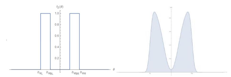
This shows a significant improvement over the ray casting method previously used on the RoboJackets RoboCup team. Figure 12 shows a comparison between the two in the case of a penalty kick. Intuitively, this method provides a more comprehensive and detailed result of the layout surrounding the chance of success.

Acknowledgements

J. Buchanan, J. Jones, J. Kamat, J. Lope, J. Ting

References

1. RoboJackets RoboCup SSL Team. RoboJackets 2017 Team Description Paper. Technical report, Georgia Institute of Technology, 2017.
2. RoboJackets RoboCup SSL Team. RoboJackets 2015 Team Description Paper. Technical report, Georgia Institute of Technology, 2015.
3. Holonomic Control of a robot with an omnidirectional drive. Raul Rojas and Alexander Gloye Forster. Technical report, University of Bremen, 2006.
4. Mora, Vincenzo Marziali, Floriano. The Zone: Advantages, Disadvantages, Countermeasures. Reedswain Inc., 2004.