RoboTeam Twente 2018 Team Description Paper
Cas Doornkamp, Zahra van Egdom, Gaël Humblot-Renaux, Leon Klute, Anouk Leunissen, Nahuel Manterola, Sebastian Schipper, Luka Sculac, Emiel Steerneman, Stefan Tersteeg, Christophe Vanderwalt, Wouter van Veelen, Haichuan Wang, Jeroen Weener, Jelle Zult
RoboTeam Twente
Abstract This paper presents the improvements RoboTeam Twente has made on the mechanics, electronics and software of their Small Size League robots, with as goal to participate in RoboCup 2018 in Montreal. Important additions are a rotating kicker and a ball sensor. The motion control of the robots has also been expanded with friction compensation and an extended Kalman filter.
1 Introduction
Last year RoboTeam Twente participated in the RoboCup Small Size League for the first time. This laid a solid foundation to build upon. Taking the results of last year into account, improvements will be made on existing features, and new features deemed useful will be added.
2 Mechanical and Electrical design
This section describes the mechanical and electrical improvements made to the robots.
2.1 Rotating kicker
One of the improvements of our robots is the addition of a rotating kicker. Being able to shoot the ball at an angle without having to rotate provides a substantial advantage. The opponent cannot use the camera data to detect the robots aiming intentions. For the implementation we looked at other teams for inspiration. A solution with a Geneva drive, like used by OP-AmP[1], has been chosen. While it limits the angles the robot can shoot at, it offers great stability of the kicker in return.
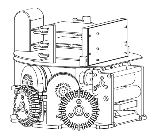
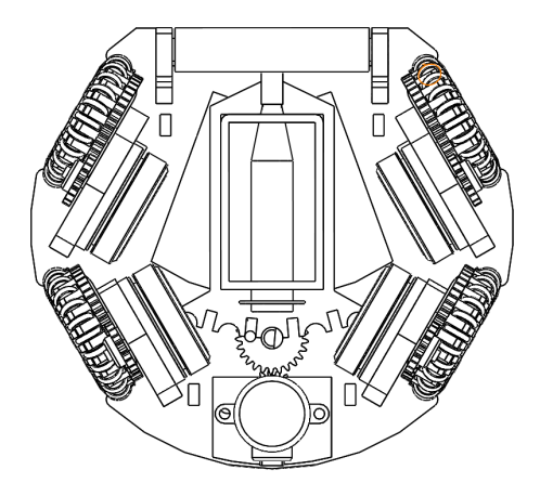
Our robots will use a rotating kicker with five possible angles. The rotating point is located in the front and the wheels in the back of the plate hold the weight of the solenoid.
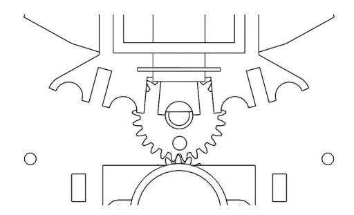
The Geneva drive is placed in the back of the robot. A gear connected to a motor drives a second gear, which on its turn drives the rotating plane. The motor has encoders installed. This allows the system to move from one locked position to the next one. This is important, since the kicker should be locked during shooting. While the encoders provide the relative location of the system, the absolute position is unknown after starting the robot. To calibrate the drive, it is rotated in one direction until a proximity sensor on the chassis measures the proximity of the drive. This is the absolute starting angle of the drive, to which the relative angle, measured by the encoders, can be added.
2.2 Chipper
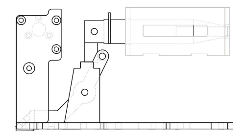
In order to get the ball off the ground, a lever is used. A solenoid is located on top of the turnable solenoid on the bottom and is directed the other way around. During activation of this solenoid, the plunger shoots to the back. Before the plunger hits the solenoid case, the handle takes the top part of the chipper with it. After chipping, both parts return to their original configuration by means of springs.
2.3 PCB layout
The electronics of the robot are divided in three boards, connected to a data and power bus via PCIE connectors. The boards are stacked on top of each other, as shown in Figure 1. The bottom board receives the battery power, delivers the required voltages to the other boards and contains the high voltage circuitry for the kicker and chipper. It also contains connections to the kicker, chipper, dribbler, ball sensor and Geneva drive. The middle board will control the wheels of the robot. It contains a microcontroller and four motor drivers, along with connections for brushless motors, HALL sensors and encoders. The top board contains the main microcontroller, communication module and IMU.
2.4 Ball sensor
An important addition to last year's design is a ball sensor that grants the robot the ability to recognize when it is in the possession of the ball without having to rely solely on the input from the vision system. For this, we opted for the STVL6180x, a small form-factor chip that determines the distance to the nearest object by measuring the time of flight. By combining an IR emitter, a range sensor and an ambient light sensor, the chip is robust to changes in eg. ball material or ambient light conditions. The main reason we chose this module is its ability to accurately measure any distance to an object from zero to ten centimeters. The chip will be placed on one side of the dribbler housing. This allows the robot to determine the location of the ball along the dribbler, which aids the robot in kicking with the rotating kicker and controlling the robot speed such that the ball is not lost when the robot is moving.
2.5 Motor controller
Motor drivers Last year's H-bridge circuitry and FPGA were replaced by a fully integrated solution, which has built-in half-bridges as well as on-board commutation and PWM generation for driving the motor phases. For this we chose the DRV10970 chip which has a simple I/O configuration and can deliver up to 1.5 A per motor.
The device offers several modes which we set as follows:
- Sinusoidal commutation which minimizes torque ripple and results in much smoother driving than trapezoidal commutation.
- Adapative drive angle adjustment, which continuously aligns the phase current to BEMF. This mode maximizes motor efficiency regardless of motor parameters, load conditions, and motor speed.
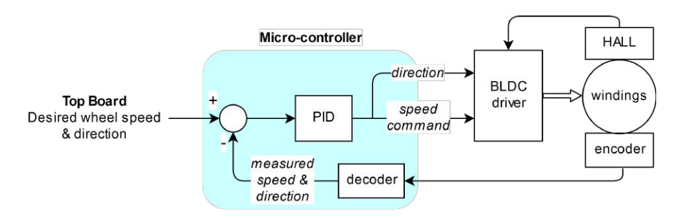
The DRV10970 chip only requires 2 GPIO pins per motor: a PWM speed command, and a signal to control the direction of rotation.
Motor speed control with quadrature encoders Last year, motor speed was estimated by measuring the time elapsed between two Hall sensor patterns. However, the resolution of such a measurement is very limited, since the Hall pattern only changes six times per revolution. This year, we wanted to implement much more precise speed measurement. For this, we use Maxon EC45 motors with built-in incremental encoders which offer a resolution of 1024 impulses per revolution. Furthermore, the quadrature output allows us to implement X4 decoding, which quadruples the measurement resolution. This allows much finer feedback control of each wheel.
2.6 Kicker driver
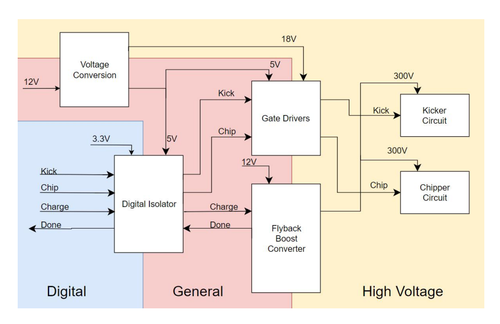
When dealing with high voltages and currents, safety and reliability are most important. In order to achieve this, the main focus has been on separation of domains. Here there are three domains: the digital low voltage domain, which the microcontrollers and other logic depend on, which is sensitive to large current or voltage spikes. The second is used for the more general purpose ICs which control most of the power circuits. The last domain is the high voltage domain which provides the large amount of power to the kicker or chipper. A visual description of this separation can be seen in Figure 6 with a functional description of the hardware. In this figure, each block that overlaps two different domains has an isolation layer to separate these domains.
In order to ensure a better reliability compared to last year's kicker, the MOSFETs that drive the kicker and chipper have been replaced with IGBTs which can handle more current and consume less power. With this, most of the components have been replaced by ICs which have internal safety measures to protect other components.
Another addition is the capacitor discharge circuitry. Whereas last year the main capacitor was discharged by activating the kicker, this year the energy will be dissipated through a resistor. This is done in order to relieve the stress on the MOSFETS driving the kicker and chipper which broke down when the voltage was getting too low; at these moments the power was mostly consumed by these MOSFETs.
3 Motion Control
This section describes the motion control improvements made to the robots.
3.1 Friction Compensation
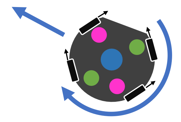
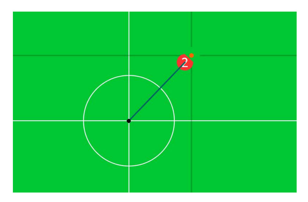
Doing precise position adjustments from standstill is difficult with last year's robot. This can be a problem. For example when another robot passes the ball, but the pass is slightly off. The receiving robot should be able to make quick adjustments within a few centimetres to get to the correct position and orientation. Another challenge in motion control is having the ability to rotate the robot while navigating to a position. Ideally the rotation should not affect the moving direction (as illustrated in Figure 7), but this also requires precise motion and fast response.
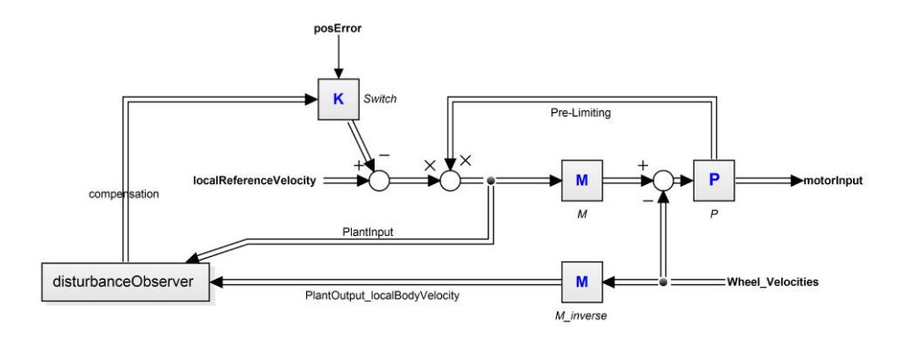
The main cause for the lack of precision is the stiction (static friction) that the robot must overcome before it starts moving. The previous approach of using PID control in each direction failed to deal with this effect. By constructing a model that includes non-linear effects like stiction and a restriction on the amount of torque that the motors can exert, we were able to test different control strategies to deal with this effect. By implementing a disturbance observer in combination with PD control, we were able to compensate for the stiction, resulting in the ability to move at low velocities from standstill. The current plan for implementing this in the low level velocity control is shown in the block diagram below (Figure 8).
A disturbance observer operates by comparing the behaviour of our system to a more ideal system. The difference is then regarded as a disturbance, which can be subtracted from the input to quickly compensate for this. We define our system to have a local velocity reference vector as input and the actual local velocity vector ($\dot{u}$, $\dot{v}$, $\dot{\theta}$) as output. This means that the control of the wheel velocities is already encapsulated in the idealized system. Note that our wheel velocity control has been changed from PI to P control, because the disturbance observer now takes over the role that the integral control had in the previous robot.
One restriction of the disturbance observer is that it does not preclude the system from becoming unstable if the ideal system model is too far off. Another problem is that if the inputs to the system become unrealistically high, the motors will not be able to provide enough torque to emulate the ideal behaviour. For this reason we decided to add what we call 'pre-limiting', which limits the reference x-, and y-velocity if one of the motor signals exceeds the maximum value. This prevents unrealistically high reference velocities from reaching our disturbance observer or saturating the motors. This part is however still under development, and might eventually be implemented differently.
However, simulations show that the strategy of applying a disturbance observer on the low level velocity control, does not seem to help in being able to rotate the robot without affecting its moving direction. We are currently investigating alternatives, including applying the disturbance observer on the global velocity level, instead of on the local velocity. Another approach that seems to already work much better is only applying the control loop on the robot body frame coordinates, and translating the output of this controller to desired torques on the motors, instead of sending velocity commands for each motor. A disturbance observer could then be implemented locally to compensate for unexpected accelerations. It remains a question how this works out in practice.
All in all, many new experiments will be necessary on the new robots to choose between different implementations of the control system that we have in mind.
3.2 Inertial Measurement Unit
To overcome the high latency of the camera system an accelerometer and gyroscope will be added to the robot. This will update the robot on current acceleration, angle and angular velocity every one hundredth of a second. This allows the robot to respond much faster to inaccuracies in the movement. The MTi-3 device by Xsens has a gyroscope/accelerometer MEMS, a magnetometer and a microchip which reads and combines their data to provide accurate movement and acceleration information. The device will communicate with the main microcontroller over a UART interface.
3.3 Extended Kalman Filter
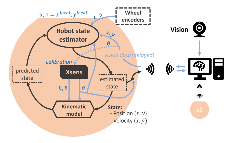
In the first version of the robot, all the information about its motion is deduced from the vision system. This yields a measured orientation ($\theta$) and a measured 2D position ($x$, $y$), which is simply differentiated over a few time-steps to obtain an estimate for the 2D velocity ($\dot{x}$, $\dot{y}$) of the robot. Although this data is reasonably accurate, the problem is mostly the relatively high delay that results from the vision measurements. We estimate between 80 ms and 150 ms of delay between sending a command to the robot and perceiving a response in the measurements (dependent on the type of camera used).
To improve motion control and for making faster decisions this delay needs to be reduced. Our solution is to add new sensors to the robot and combining these by designing an Extended Kalman Filter (EKF). These new sensors consist of encoders for each wheel, yielding wheel velocities, and the Xsens MTI-3 module, an enhanced IMU that also enables accurate tracking of the yaw (orientation).
The first diagram (Figure 9) shows the preferred setup of the EKF that will be used for our robots. The Xsens module is equipped with accelerometers, gyroscopes and magnetometers. The accelerations measured by the accelerometers in the u and v direction (which are coordinates in the robot frame) can be used in a kinematic model to make fast predictions of where the robot will move next. Note that the Xsens chip is placed at the centre of rotation of the robot, such that the centripetal acceleration and other unwanted accelerations will not be measured. The data from the gyroscopes and magnetometers are already combined by the Xsens module itself to get a fast and accurate estimate of the robot orientation ($\theta$). It will have to be tested whether this estimate is reliable enough, considering the possible disturbance caused by magnetic fields produced by the circuitry and the solenoid. It will also still be necessary to perform a calibration when the system is started, using the orientation outputted by the vision system. However, the disadvantage of the vision data being delayed does not play a role in this case, because the calibration will be performed while the robot stands still.
The kinematic model makes a prediction on the state one step into the future. The state is a combination of the global 2D position and velocity. When new measurements from vision and the wheel encoders come in, these can be combined with the predicted state to give the best estimate of the state. The uncertainties of all states are tracked in covariance matrices, which is necessary for comparing the reliability of the measured and predicted quantities. The estimated state will be both used in the control of the robot, as well as send back to the central computer for decision-making. The orientation outputted by the Xsens module is then merged with the state before sending it back to the computer. In that way each robot receives vision information from the computer and sends back the best estimate of its own pose $(x,y,\theta)$ and velocity $(\dot{x},\dot{y})$.
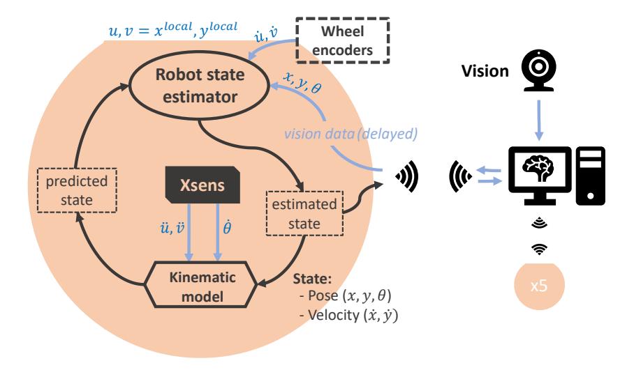
If the magnetic measurements turn out to be too unreliable, the EKF will be constructed in a slightly different way, as illustrated in the second diagram (Figure 10). The difference is that the state includes the orientation of the robot, and the angular velocity is received from the Xsens module instead of the yaw. The vision data of the robot orientation now becomes the only source for referencing the yaw, which will suffer from the relatively high delay of the vision system. If the amount of time-steps in this delay is well known and not too large, it will be possible to partially compensate for this [2].
4 Communication
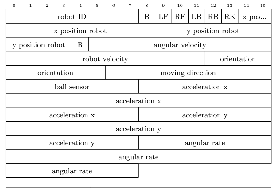
The design of the packets used for communications between the tactics computer and the base station has been altered. The packets send to the base station facilitate controlling the rotating kicker (Figure 11). The packet send from the base station to the tactics computer provides status information about the robot. Debug information can be requested, giving insight in the measurements done on the robot (Figure 12).
Dribbler speed The new packet design allows us to adjust the speed at which the roller rotates, which will help to improve the control of the robot. We expect this to have great effect in scenarios such as automatic ball placement.
Kicker angle The kicker angle field is used to indicate under which angle the robot has to shoot. Options are -20°, -10°, 0° (straight), 10° and 20° as per the physical possibilities described in 2.1. The robot will never kick or chip if the kicker is not in its desired state to prevent shaky passes and unnecessary damage to the rotating kicker device.
Debug information Debug information from the base station can be requested by setting the "Debug" bit in the packet. This provides the tactics computer with information about the acceleration and angular rate of the robot.
Extra information Extra information can be send to the base station by setting the "Extra" bit. When this bit is set, the computer includes information about the position and orientation of the robot as perceived by the camera in the packet. This information can be used in the future for motion control calculations done on the robot.
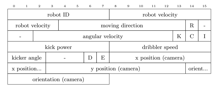
Communication control options sent from tactics computer to base station
| Rotating direction | The desired rotating direction of the robot. |
|---|---|
| Kick | Kick as soon as the ball has been detected. |
| Chip | Chip as soon as the ball has been detected. |
| Kick Immediately | Kick or chip without waiting for the ball sensor. |
| Debug | Request debug data from the robot. |
| Extra | Indicate that extra information will be send with this packet. |
5 Automatic Ball Placement
Unlike last year, this year the competition will be divided into two divisions: division A and division B. In order to be able to participate in division A, robots needs to be programmed to perform an automatic ball placement (ABP). During a match, the referee can assign a team to perform an ABP. The team assigned to the task is required to send a robot to place the ball at a specified location within 15 seconds and with a maximum error of 0.1 m.
The ABP has been implemented using behaviour trees, as described in last year's paper [3]. To perform an ABP the robots are assigned one of two roles. The first role is the ABP role. This role is assigned to the robot that is closest to the ball (from now on called ABP robot), to make sure the ABP is performed as fast as possible. The other role is assigned to the other robots. This role instructs the robots to move away from the ABP robot. This way the ABP robot only has to focus on keeping the ball and does not have to take robot avoidance into account as well.
The role of the ABP robot is constructed with a decision tree (Figure 13) and contains two skills. The first skill makes sure the robot gets the ball while the robot is located between the ball and the location where the ball needs to be placed (Figure 14). The second skill makes the robot drive in backwards direction with its dribbler activated until the ball is at the right location. The robot does this with a reduced speed to prevent loss of the ball. Driving backwards instead of forwards is favourable because it makes getting the ball when it is close to the border easier and the chance of losing the ball is smaller.
Besides the skills, the tree also contains a sequence and a RUS (Repeat Until Success)(Figure 13). An arrow is used in the figure as the symbol for the sequence. The function of the sequence is that it executes its children (here the two skills) in order until one of them fails. If the sequence is repeated after it stopped, it will start again with executing its first child. As its name already suggests, the RUS will repeat the sequence until everything succeeded. If this is the case the ABP is done and the robot can go back to the right position.

References
- OP-AmP. "OP-AmP 2017 Team Discription Paper". In: (2017). url: https://www.robocup2017.org/file/symposium/soccer_sml_size/Robocupssl2017final9.pdf.
- T.D. Larsen et al. "Incorporation of time delayed measurements in a discretetime Kalman filter". In: 4 (Jan. 1999), 3972–3977 vol.4.
- RoboTeam Twente. "RoboTeam Twente 2017 Team Description Paper". In: (2017). url: https://www.robocup2017.org/file/symposium/soccer_sml_size/Robocupssl2017-final24.pdf.