2018 Team Description Paper: UBC Thunderbots

Mathew MacDougall, Gareth Ellis, Amy Hashemi, Emma Jackson, Oon Chu Lip, Nicolas Ivanov, James Petrie, Khashina Tonks-Turcotte, Chantal Sousa, Kenji Lai, Bowen Xu, Qiqi Li, Eric Goto, Dana Deutsch, Anthony Buonassisi, Marcus Lee

The University of British Columbia

www.ubcthunderbots.ca

Abstract This paper details the design improvements the UBC Thunderbots has made in preparation for RoboCup 2018 in Montreal, Canada. The primary focus was to develop the capability for our robots to pass during gameplay. To do this, we focused on improving our existing mechanical and electrical systems to accurately execute actions needed to send and receive passes. The secondary focus involved building upon the existing artificial intelligence to utilize these passing capabilities.

Introduction

UBC Thunderbots is an interdisciplinary team of undergraduate students at the University of British Columbia. Established in 2006, it pursued its first competitive initiative within the Small Size League at RoboCup 2009. The team has consecutively competed in RoboCup from 2010 to 2017 and is currently seeking qualification for RoboCup 2018. Over the years, it has made significant developments of its team of autonomous soccer playing robots. This paper will outline the progress in implementation of the current model of robots, focusing on the mechanical, electrical and software components with particular emphasis on the software systems.

Mechanical Design

This year, we have developed several new mechanical systems that will be implemented in a prototype robot to be tested as an integrated system during the summer of 2018. Upon successful testing, we plan to implement these new designs for the following years competition.

2.1 Chipper and Solenoid Redesign

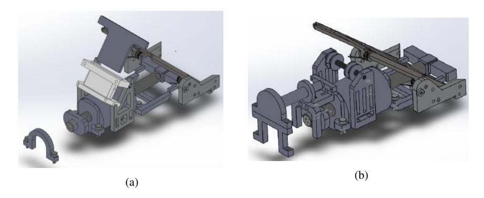
Currently, our robots contain two solenoids used to enable kicking and chipping. In the current construction of the robot, this mechanism is placed centrally at the bottom of the robot where the current free space in the body is around 18 cubic inches, and the current orientation of the chipping solenoid occupies 2.58 cubic inches. Though it takes very little space, the orientation of the chipper solenoid is prohibiting the use of the available free space. This inefficient use of space forces other components of the robot to be placed further from the ground and, in turn, causes the robot to have a higher centre of mass. We are redesigning these kicking and chipping mechanisms to be more compact and use the available space more efficiently. This will enable us to reduce the height of the robot in the future and lower the robots centre of mass.

The new design aims to improve these issues by creating a modular pulley system, where the current rectangular solenoid is replaced with a small cylindrical one that is stacked on top of the existing plunger stopper at the rear of the robot. This not only increases the efficiency of the space usage, but also allows us to decrease the height of the chipper and thus reduce the centre of gravity of the robot. The chipper arm will remain mostly unchanged, except for a decrease in height, and the addition of two holes where the actuation cables connect. Underneath the actuation point will lie two pulleys where the cable will form a 90 angle to the chipper arm, replicating the forces that currently actuate the chipper.

When the solenoid is energized, it will cause a cylindrical ferromagnetic plunger connected to two wires to be pulled into the magnetic field of the solenoid. The other ends of the two wires are connected to the chipper plate via two small holes drilled into the top of the plate. This will trigger the chipper plate to pivot and chip the ball. It is estimated that through this redesign, we will be able to reduce height chipper assembly by 1.5 cm without a decrease in capability of chipping, freeing up space within the center cavity of the robot. Through this design we will also be standardizing the solenoids that will be used for future robots to increase the accuracy of our chipping. The design also helps the issue with slippage that the back wheels have been experiencing during acceleration, as weight will be shifted significantly to the rear portion of the robot. This assembly shifts the center of gravity of our robots and frees up additional space for potential electrical expansion in the years to come.

2.2 Dribbler Roller

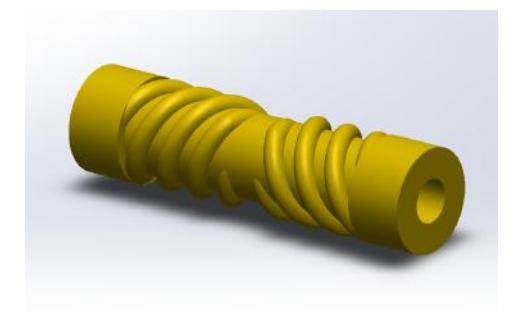
To enable our robots to kick more accurately, we have developed a dribbler mechanism to center the ball while the dribbler is rotating. Our design, shown in figure 2.2, utilizes screw-shaped etches on the dribbler instead of using a conventional cylindrical tube. The dribbler is made using a 3D-printed mold. These etches push the ball towards the centre of the robots kicking mechanism while the dribbler motor is running.

To validate this design, two experiments will be carried out. The first experiment will be to determine the best material to be used on the dribbler. Materials that are being considered are polyurethane of different shore hardnesses. The ideal material will have the highest grip on the ball while minimizing ball rebound. The second experiment will be determining the optimal design for the dribbler. The factors being varied here are the radius and angle of the thread. The best design can center the ball within the shortest time possible. The result of both of these experiments will give us the final specifications of the dribbler.

2.3 Break Beam Mount

The latest iteration of the break beam design is susceptible to misalignment from various factors such as the ball impacting the structures surrounding the break beam or direct contact with the break beam structure. It is also possible for the vibrations from the robot in normal operation to misalign the sensor. The structure to hold the break beam sensor is currently designed so that the sensor is housed in a metal structure that clamps down on the sensor when a screw is tightened. The problem with this design is that force is only applied in one dimension, allowing unrestricted movement in the other directions.

To address this problem, we have created a new design that incorporates the downward clamping aspect from the current design, but also constraints linear or rotational motions of the break beam sensors within the housing structure. The new design utilizes an extra component that is shaped like the sensor to clamp down on the sensor from an angle perpendicular to the main clamp, thus restricting the sensors lateral and vertical movements.

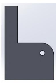
In our design we utilized a deprecated hole on the baseplate that was used in a previous iteration of the mechanical design. This puts our redesigned component situated on the outer side of the dribblers L-shaped side plates, seen in figure 2.3. There are a few reasons for this design decision. First, the side plates act as a support in the case that the ball impacts the frontal area of the robots shell. The side plates will also absorb shock from an internal impact and reduce the effect of imparted forces on the sensors alignment. Another reason is that by utilizing the deprecated hole, the manufacturing of a design with our given spatial limitation is made substantially easier since we can rely on preexisting components and features on the robot for stability and support.

In figure 2.3, a fully and properly dimensioned CAD model of our design is shown. The next step is to prototype our design using a water-jet cutter and test it to see if the part improves the performance of the break beam sensor. Other factors such as ease of assembly and disassembly will be also be tested.

2.4 Dribbler Mounting Redesign

In the current generation of robots, the dribbler is mounted on the base-plate using screws that pass through the steel base-plate and are threaded into the aluminum dribbler. For the upcoming prototype robot, we are redesigning the mounting system to eliminate the issue of stripping the aluminum taps and to improve assembly and disassembly procedure for quick and easy access. Experience in past competitions has shown that tapped holes in aluminum are not an ideal solution and using nuts makes the assembly process longer. Eliminating the use of the tapped holes will increase the lifespan of the dribbler and its ability to withstand the impact from the ball without the need for replacement parts. Replacing the taped aluminum and screws will make the disassembly, repair, and reassembly of the robots during a competition more efficient, and the parts wil.

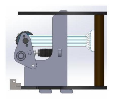
To achieve these goals, we have designed two potential mounting systems, seen in figures 2.4a and 2.4b, for the redesigned dribbler. Both designs use tabs or hooks in the upper and lower edges of the side plates and corresponding slots in the baseplate and mid-plate seen in figure 2.5a to replace the screws and tapped holes. The side plates are fully constrained by the weight of the upper half of the robot and the screws pushing into the supporting columns. This will allow for a quick-release system, by partially loosening the screws holding down the mid-plate and sliding the dribbler forward, which is more efficient than fully removing several screws from tapped holes as well as raising the middle plate. We plan to create physical prototypes of both designs to determine which design is more effective at holding the dribbler stationary in game play conditions with ball impacts. The final design will be implemented with the redesigned dribbler.

2.5 Internal Gearing

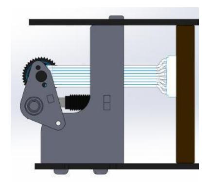
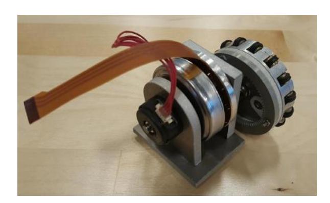
The redesign of the drivetrain has continued since 2017 [1]. The new internal spur gear, driving gear, and wheel assemblies have been assembled on to a test piece of aluminum. The encoder has been moved to the backside of the motor because it can no longer fit where it was originally located due to the distance between the cantilever shaft holding the wheel and the motor shaft decreasing. Future plans include ordering and assembling three more of these assemblies, installing them into a robot and testing. After this, a new motor mount that can be used in any wheel location will be designed to reduce manufacturing costs and machining time.

2.6 Omni-Wheel Optimization

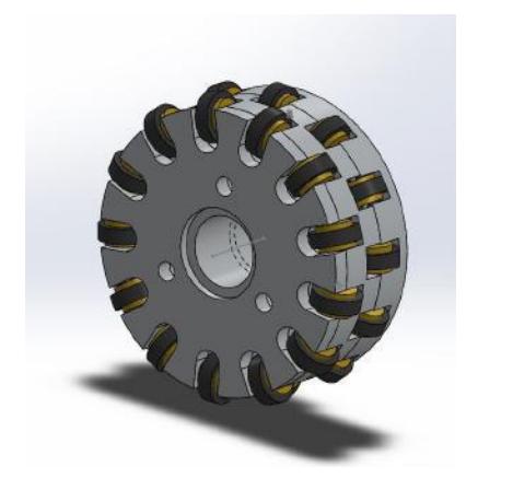
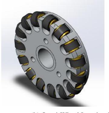
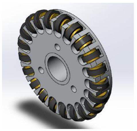
Currently, the usage of single layered omni-wheels allow our robots to traverse the standardized playing field with minimal movement constraint. The current omni-wheels use fifteen 5 mm rollers, leaving gaps of 3.5 mm between each roller. The excess space between these rollers have proven to be problematic.

In the existing design, when the rollers contact the ground the rollers are forced upwards into the wheel well, leaving the wheels only 0.3mm off the ground. As the wheels rotate, this lowered height causes the parts of the aluminum to strike the ground before the following roller. The parts of the aluminum wheels that begin to contact the ground have a lower coefficient of friction with the playing field, causing the robots to slip on the playing field. Slippage is undesired as it causes errors in our robots optical encoder based dead reckoning system.

We chose to address the problem with three design iterations. The first, shown in figure 2.7a utilized a second row of omni-wheels that were positioned so they would be present where the first row did not contact the ground. This would allow the wheels to have a much more consistent contact plane to the playing field. The second iteration considered, (figure 2.7b), used the same number of omni-wheels, but had wider rollers. This would have a greater area of contact with the ground. The third iteration (figure 2.7c) implements a larger number of rollers in the same space of the omniwheel, decreasing the space in between the rollers and the risk of the wheels touching the ground. This design increases the numbers of rollers from fifteen 5mm rollers to twenty-one 5mm rollers, reducing the space in between the rollers by 1.25mm to a spacing of 2.25mm. Each design considered will directly address slippage seen in the robots but also prevent the motors from stalling, thereby, increasing the overall efficiency of the robot. The larger number of omni-wheels also reduces vibrations when the robot moves, which makes software designed for movement easier to implement. Better control over the robots movement will allow for the team to more effectively execute software written for the robots movement and position, increasing the potential for more complex plays.

The larger number of omni-wheels reduces vibrations when the robot moves, which makes software designed for movement easier to implement. Better control over movements will allow for the team to more effectively execute software written for the robots movement and position, increasing the potential for more complex plays.

2.7 Shell Mounting

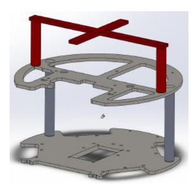
During previous competitions, we have experienced radio problems where our robots become unresponsive when far away from our radio dongle. We suspect this may be caused by signal power loss due to the presence of parasitic antennas, in the form of metal components in our robots mechanical frame, near our robots radio antenna. The one large metallic crossbar, shown below in figure 2.8, near the radio antenna that may be contributing to the loss in signal power. The purpose of this metal crossbeam is to secure our robots shell to the interior frame of the robot.

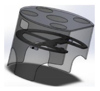
To help reduce signal power loss due to parasitic antenna, we have removed this crossbar from the robot and designed the shells to mount to the robots frame without relying of this crossbar. With this shell mounting system, our shells are mounted by slipping it over two spring plungers installed on the side of the robot, this change will reduce the potential for radio interference, decrease the weight of the robot, and lower its centre of mass. The new shell is shown below in figure 2.9.

Software

This section covers the software improvements made to our robot systems.

3.1 New Shooting Primitive

To keep up with the continually improving strategy and gameplay in the league, particularly focusing around offense, we have added new robot primitives to our set of movement primitives initially presented in [2]. We noticed that offensive plays tend to be highly dynamic in their decision making, because the best location to pass or shoot can change rapidly at any time. Therefore we developed a new shooting primitive that is more suited for rapidly changing decisions when the robot is already close to the ball, rather than open-field play with a dynamic ball.

The new primitive combines control elements from our previous shooting and pivoting primitives outlined in [3], to allow the robot to quickly reposition about the ball to adjust for a new shooting target. The robot will adjust its distance from the ball as it pivots around it, maintaining a small buffer initially and reducing the distance to transition the final approach into a shot. Compared to our existing shooting primitive which would need to completely fall back and re-align with the target, this is much quicker and more space efficient.

3.2 Optimizing the Move Primitive to Reduce Wheel Slip

To improve the movement of our robots, we have applied an optimization to our move primitive described in [3]. Previously, when robots were moving along a straight line to their destination their orientation was not explicitly controlled while they were in transition. However, due to the holonomic layout of the robot wheels opposing forces can be generated as the robot moves. We observed this typically results in one or more wheels slipping. As a result, the robots do not follow the desired movement trajectory and errors are introduced to the robots encoder based dead reckoning system.

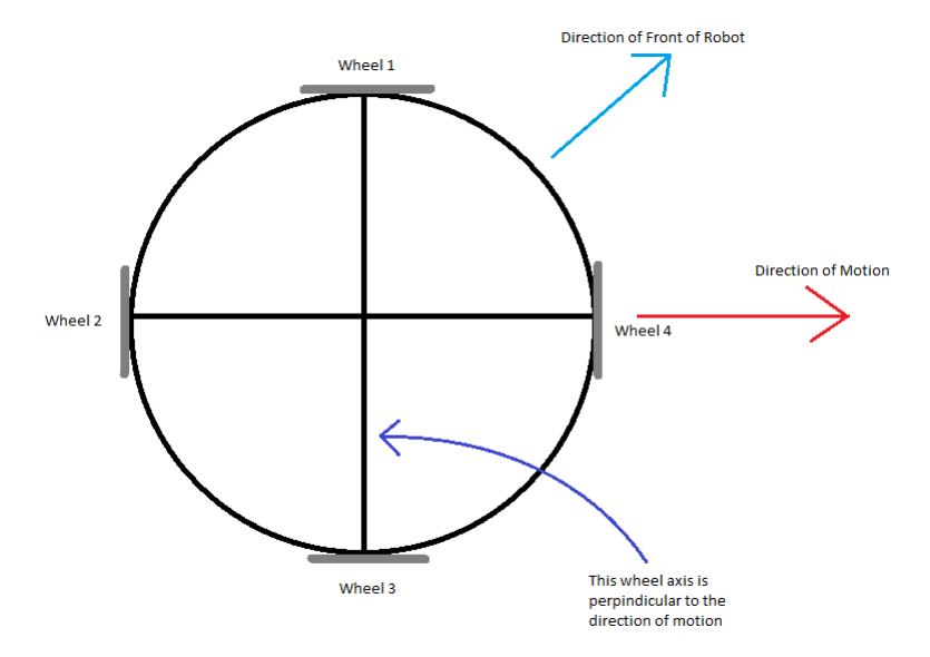
To address this issue, the robots now try to orient themselves with their direction of travel as much as possible. By making one of the wheel axis parallel to the velocity vector of the robot, two wheels can drive the robot and the other two are perpendicular to the direction of travel and coast on their omni-wheels. This is illustrated in figure 3.1. This results in a minimal amount of opposing wheel forces and allows the robots to move in a more controlled fashion.

3.3 Spline Movement

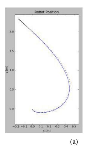
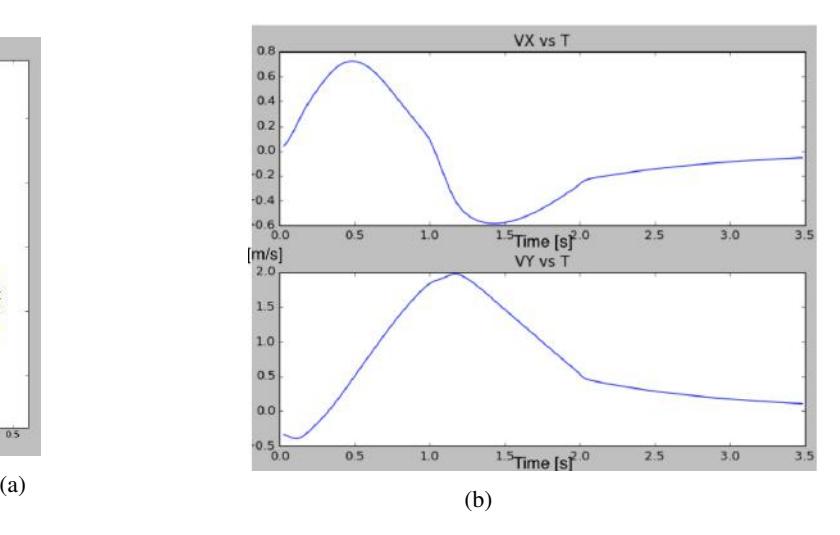
Taking advantage of the movement primitive framework [2] and vision streaming [1], the onboard controller is now in a position where it can handle the control of the entire robot trajectory. In previous years we either used a control PC PD controller, or more recently we frequently transmitted "line primitives" in changing directions. The purpose of this new development is to enable precise movement planning and control so that the robot arrives at a location at a specified time with a specified velocity, which is very useful for ball interception mechanics. Using wheel encoder information fused with latency corrected camera data [1] the feedback loop is much more accurate and faster on-board the robot than using the host PC.

A Bezier curve was a natural choice given the requirements. A Bezier curve is a cubic spline which is defined using four control points. These control points allow for smooth, physically achievable paths to be generated in an efficient manner.

$$C^0 = \text{robot starting point}$$ $$C^1 = C^0 + \text{initial stopping distance}$$ $$C^2 = C^3 - \text{final stopping distance}$$ $$C^3 = \text{robot end point}$$

By setting the middle control points based on the stopping distance corresponding to the initial and final velocity, the path generated is achievable and extremely easy to compute. An added benefit of using a Bezier curve is that only the control points need to be transmitted over the radio to encode the entire path.

Given a Bezier curve has been selected by the control PC, it is transmitted over the radio along with the final velocity and arrival time. The firmware then plans the future velocity along the entirety of the path such that the input requirements are met and the robot doesnt deviate from the path due to excessive centripetal acceleration. This is accomplished by discretizing the path and using a model of the robot that can determine the greatest acceleration achievable given the current robot velocity for each segment.

Using the planned trajectory, the robot then begins its motion. The segments are required to be completed in order, each with a "finish line" used to determine when to follow the next segment. The applied acceleration in the direction of travel is the sum of the planned acceleration and a proportional controller based on the difference between the actual and planned velocity. In the tangential direction the acceleration is the sum of the calculated centripetal acceleration for the current velocity and curvature, as well as a PD controller using the tangential displacement from the path.

If along the path the current velocity ever deviates significantly from the plan or the intermediate arrival time doesnt match the schedule, the entire trajectory is re-planned. Large positional displacements are left to the control PC to decide if a new plan is necessary.

3.4 Bezier Navigator

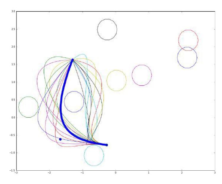
This navigator is intended to provide physically achievable, smooth paths when dealing with limited obstacles. A considerable amount of the time when planning a path, there are not significant obstacles in the way, especially when near the destination, where accurate movement is often more important. The benefit of this navigation algorithm is that it factors initial velocity into the decision, and it is computationally efficient when dealing with sparse sets of obstacles.

This navigator functions by performing a guess-and-check search on various Bezier curves, starting with the fastest arrival time, then checking slower paths [4]. Each of the curves attempted has the second control point in a location based on the initial velocity. If a path in the limited search space is found, the spline primitive is executed. In the failure condition, a more sophisticated algorithm like RRT or A* is used.

3.5 Deterministic Path Planning via Multi-Resolution Graphs

This year we are developing a new path planner to overcome the drawbacks of the former system. Our previous algorithm was based off of Rapidly-Expanding Random Trees, which had several shortcomings. Firstly, the paths returned by the algorithm were non-deterministic due to its random nature. Furthermore, the algorithm is not guaranteed to find a valid path to the destination if one existed. We observed the algorithm could get stuck if an expanding branch was sufficiently blocked, due to the biased generation of segments in the direction of the destination.

Our new approach revolves around representing the field as a graph. This is because with a generic graph representation of the field, we have a diverse selection of graphsearch algorithms to utilize for generating a path from the start node to the destination node. Our algorithm of choice is the A* algorithm, due to it being both optimal and complete. The list of nodes returned by the A* algorithm will be simplified into a path made up of the fewest straight-line segments possible.

The main challenge of this approach is the representation of the graph, because of the tradeoffs between memory usage, algorithmic complexity, and precision. Ideally our graph would contain many nodes at as high of a resolution as possible so that we can accurately represent our final destination, and tight paths around obstacles. However, our ability to store this many nodes is limited by the system we are operating on. For example, storing a grid of nodes with 1mm separation for a 9x6m field takes on the order of several gigabytes of memory. This leads to unusably slow graph generation times. Furthermore, traversing this many nodes in a graph-search algorithm takes a significant amount of time, even with more optimal algorithms like A* traversing as few as possible.

Our solution to balance the tradeoffs as to use multi-resolution graphs. Since most of the field is sparsely populated with obstacles, those areas of the graph do not need the extreme resolution that locations, such as the destination would, to produce satisfactory paths. Yet, we still want the flexibility of having greater node density in areas where more accurate and precise maneuvering would be necessary, such as around obstacles. Multi-resolution graphs allow us to combine the desired characteristics of both solutions, reducing our memory usage and runtime by maintaining fewer nodes, while still allowing for precise path representation when necessary.

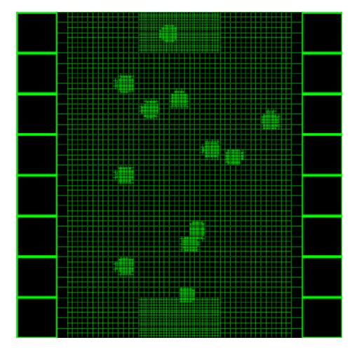
Our container for storing the multi-resolution graphs is an n-ary tree, where each vertex is a subgraph of its parent vertex, with the lowest level of nodes being the nodes in the graph. By extension, these lowest level nodes are a representation of the physical search space, in this case the field. This multi-resolution graph concept is illustrated in figure 3.5. The tradeoff between memory usage and algorithmic complexity comes with the function for finding neighbours. With a tree of low depth, in the extreme case a single graph with no sub-graphs, we must represent the entire field at the maximum fidelity required for any given point on the field. While such a graph makes it very easy to find neighbours, as they would just be adjacent cells in a 2D array representation, this is where we enter the realm of multi-gigabyte memory usage.

To reduce this memory footprint, the top level graph is set to a relatively low resolution. For example, nodes at this level are 10cm apart on the field, and sections of the graph that require higher resolution are split into sub-nodes, with each sub-node being a higher resolution sub-graph of part of the field. When searching for the neighbours of a given node in a subgraph, we now search first in the nodes current sub-graph. If any of the the neighbours cannot be found, for example if the node is at the edge of the subgraph, then we search through the parent graph of this subgraph. This is performed recursively at each level in the graph up to the top-most graph. For a tree of depth d and max graph size n, we will have to search from some node up to the top-most graph, and then back down the tree again. At each graph we visit (of which there are $2 \times d$) we must perform a O(log(n)) search to see if this graph contains (directly or in a sub-node), the neighbour were looking for. This results in a $O(d \times log(n))$ runtime to find a given neighbour of node. This scenario, however, is unlikely as the majority of the nodes are not at the edges of a graph. For a tree where each subgraph is square and contains 100 nodes (n=100), only the edge nodes, of which there are 36, will take $O(d \times log(n))$ to look up one of their neighbours (with the corner nodes having to look up two neighbours), with the rest being contained on the subgraph. All other nodes in the graph will take O(1) to lookup their neighbours (as they are directly adjacent in the subgraph). Hence, we will only have the worst case runtime for 40 of the possible neighbours in the graph, or $\frac{40}{100\times4} = 0.1%$ of cases, with all other lookups being O(1). This still assumes however, that we must traverse the entire depth of the tree in order to find the neighbour. With intelligent placement of higher resolution subgraphs, for example by having a Gaussian Distribution of resolution around points of interest, this time can be reduced even further.

Because this new planning algorithm will be guaranteed to find a path if one exists, we expect to use it primarily as a fallback for the Bezier Navigator discussed in the previous section. Should the Bezier Navigator fail to find a path, this graph-based planner will be used so that a path can still be returned. This will allow us to experiment with other planning algorithms that sacrifice completeness, while always having the guarantee that we can return a path.

3.6 Particle Filter

With the increase in gameplay speed in the league, it is more important than ever to be able to accurately and responsively track the ball on the field. In recent years, our team has observed slow reaction speeds from our robots, particularly to shots and passes, and determined this was due to an unresponsive ball filter.

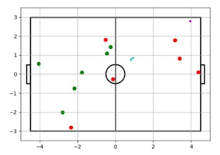
Our previous system was based on a Kalman filter, which was exceptional at modeling the linear motion of the ball but not the situations where the balls motion broke this linearity. For example, the Kalman filter would accurately track a ball moving in a straight line across the field. However if this ball bounced off a robot, the Kalman filter would still report the ball as moving along is previous path for a short amount of time, due to how much confidence it held in its linear model of the ball. This resulted in our robots reacting slowing to scenarios such as shots on net, because by the time the filter reported the ball as moving towards the net, it was already nearly there. A simulated example using game logs can be see in figure 3.6. The ball was originally kicked from the magenta location in the top right, and is still reported to be there by our old filter, while SSL-Vision data is shown nearly halfway across the field in cyan.

We chose to implement a Particle Filter due to its strength at tracking non-linear motion. Because the filter does not contain an internal movement model that it expects the ball to follow, it is more adaptable to suddenly changing ball velocities. The filter works by generating particles, which are Cartesian points with a certain weight, around every potential ball location as reported by SSL-Vision. A weight for each particle is calculated using an evaluation function, that scores particles higher that are close to an SSL-Vision detection, close to the balls previously predicted position, and close to the balls previous position. After the particle weights are updated, the top 10% of particles are kept and the others are discarded. These selected particles are then used as base points to generate more particles around. Once the particles are generated, they are evaluated again and this cycle continues for several iterations. Each iteration, the particles will converge towards the most likely location of the ball as determined by the evaluation function. After several iterations, the final set of points is averaged to give the final ball position, which is returned to the rest of the AI system.

The new filter has proven to be very successful, tracking a variety of non-linear ball trajectories with very high accuracy and responsiveness. We have reduced the response latency of the filter from 1 second to nearly 30ms.

Control

This section covers the control systems for the robots.

4.1 Motor Modeling and PID Controller

Currently, our robot uses a positional bang-bang controller to regulate motion between two points. While this method of control is simple to implement and able to move the robots around the playing field, it is relatively ineffective when trying to move small distances. In order to achieve the short, precise movements needed to receive passes, we are developing a PID controller for our robots. We hope that this controller will enable us to smoothly travel small distances and overall have more control over the movement of the robot.

To create our PID controller, we have begun by developing a physically accurate model of our robot. Once a physical model of the robot is constructed, we plan to use MATLAB and Simulink to tune the gain parameters of our controller.

The first portion of our model is a model of our motors. We currently use Maxon EC 45 brushless DC motors. Using the data sheet, we constructed the following transfer function translating voltage to angular velocity:

$$\frac{\dot{\Theta}(s)}{V(s)} = \frac{K}{(Js+b)(Ls+R) + K^2}$$

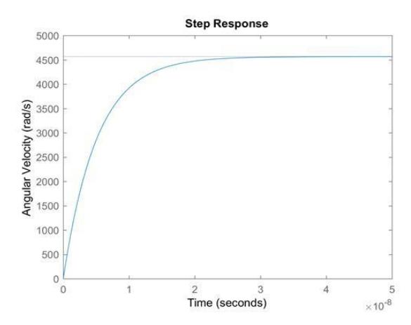
J represents the moment of inertia (92.5 $\text{gcm}^2$), B is the viscous friction constant (which in most cases is small enough to be ignored), L is the armature inductance (0.56 mH), R is the armature resistance (1.2 Ω), and K is the motor torque constant as well as the electromotive force constant (25.5 mNm). Simulations of this transfer function using MATLAB are shown in figure 4.1.

Simulations of this transfer function for a voltage change from 0 to 3V using MATLAB are shown in figure 4.1. This is verified through physical tests with the encoder data logged on the robot.

However, the angular velocity is not very useful to the simulation model, because the simulation model needs the torque the wheels apply against the floor in order to calculate accelerations on the robot. Instead of having a closed loop transfer function like the one shown above, were going to model the motor as a simple inductor and resistor in series. From the electrical properties of these components, we can implement a discrete model that takes in angular velocity to factor in rpm and viscous motor friction, and outputs a current, which is directly proportional to Torque, which the other parts of the simulator can use.

Conclusion

We believe that the design changes detailed above will lead to significant improvements in performance. We look forward to putting the changes into action at RoboCup 2018.

Acknowledgements

We would like to thank our sponsors, as well as the University of British Columbia, specifically, the Faculty of Applied Science and departments of Mechanical Engineering, Engineering Physics, and Electrical and Computer Engineering. Without their continued support, developing our robots and competing at RoboCup would not be possible.

References

1. C. Y. Bai, W. Gong, B. Hers, B. Hsieh, R. De Iaco, Y. Z. Ju, B. Jury, B. Long, K. L. Lu, J. Petrie, K. Tonks-Turcotte, C. Xie, D. Yang, R. Zaari, K. Zhang, and K. Zhang, "2017 Team Description Paper: UBC Thunderbots," 2017.
2. S. Churchley, R. De Iaco, J. Fraser, S. Ghosh, C. Head, S. Holdjik, N. Ivanov, S. Johnson, F. Kalla, A. Lam, B. Long, K. Lu, S. Ng, K. Peri, J. Petrie, E. Roach, W. Y. Su, B. Wang, C. Xi, K. Yu, and K. Zhang, "2015 Team Description Paper: UBC Thunderbots," 2015.
3. R. De Iaco, S. Johnson, F. Kalla, L. Lu, M. MacDougall, K. Muthukuda, J. Petrie, M. Ragoonath, W. Su, V. Tang, T. Tsu, B. Wang, B. Whyte, C. Xie, K. Yu, E. Zhang, and K. Zhang, "2016 Team Description Paper: UBC Thunderbots," 2016.
4. E. Schluntz, "Real Time Path Planning with Trajectory Libraries."
5. "GPUs To Mars: Full Scale Simulation of SpaceX's Mars Rocket Engine," 2015.