ZJUNlict Extended Team Description Paper for RoboCup 2018
Lingyun Chen, Lisen Jin, Cheong Weng Lon, Licheng Wen, Jianyang Gu, Jiacheng Li, Tianqing Fang, Rong Xiong
National Laboratory of Industrial Control Technology; Zhejiang University
http://www.st.com/en/microcontrollers/stm32f4-series.html?querycriteria=productId=SS1577 · http://www.st.com/en/evaluation-tools/nucleo-f767zi.html · http://wiki.robocup.org/images/b/bc/Robocupssl2017-final21.pdf
Abstract ZJUNlict has been participating in Robocup for fourteen years since 2004. In this paper, we summarizes the details of ZJUNlict soccer robot system we have developed in recent years. We emphasize on the main ideas of designing the robots hardware and our software systems. Also, we will share our tips on some special problems. We develop a better sensor fusion in electronics, and optimize ball-catching ability as well as flat-shoot stablility, which have great effect on court. In software, we update our vision module as well as motion control method, and adopt a new parameter self-adaption module in our system.
Introduction
Our team is an open project supported by the National Lab. of Industrial Control Technology in Zhejiang University, China. We have started since 2003 and participated in RoboCup during 2004-2017. The competition and communication in RoboCup games benefit us a lot. In 2007-2008 RoboCup, we were one of the top four teams in the league. We also won the first place in Robocup China Open in 2006-2008 and 2011. We won the first prize in 2013 and 2014, which is a great inspiration to us. In recent three years, we have stayed within top 3 in RoboCup games.Also, we incorporate what we have done in recent years in this paper.
Our team members come from several different colleges, so each member can contribute more to our project and do more efficient work.
Hardware
2.1 Mechanics
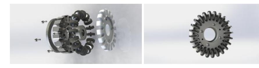
New Omni-directional Wheel We redesigned a brand new omni-directional wheel, which to some extend overcame the polygon effect. As we all know, the reason why our robot can move in multi-direction is that we use the omnidirectional wheel. And there is actually quite some problems in it. One of them is the polygon-effect which due to the shape of the section of the wheel. It is not perfectly round. However, when we increase the number of small wheels in a single big wheel, the section become more like a circle.
The wheel we used before contains 16 small wheels in every single big wheel, and the section can be considered as a sixteen-deformation. When the robot moves in a high velocity, the vibration becomes non-ignorable, and is always account for the overshoot.
With the prototype of 20 small wheels and 24 small wheels, we proved that the more small wheels we have in single big wheel, the more stable it will be. However there are many holdbacks when we try to put more small wheels in one single big wheel, such as, the intervention between small wheels. The solution will be making the small wheel small.
Thus, we will be using the 24 small wheels version of robot for the next few international cups.
Stabilize Ball Catching
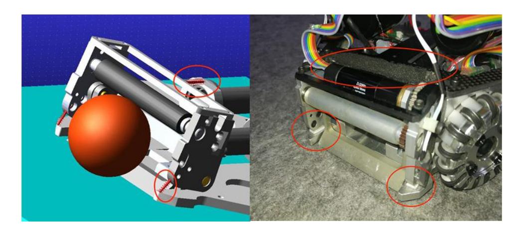
Study damping relations to improve catching performance. We added quite a few tiki-taka into our strategy this year. To catch the ball coming from high speed, you need to design a better cushion to absorb the kinetic energy of the ball. In the past, we put a spring behind the mouth, but the problem with the spring is that although it stores energy, it still releases the energy and bounces the ball out. With qualitative analysis and Computer Aided Analysis with ADAMS, we know that in order to absorb and consume the kinetic energy, the key is the need for a damping system. We changed the spring behind the mouth to a sponge and padded a 3M glue under the mouth to create a bi-directional damping system. It greatly improved the catching performance of the mouth by matching the two non-linear materials.
Solve Shovel Vibration
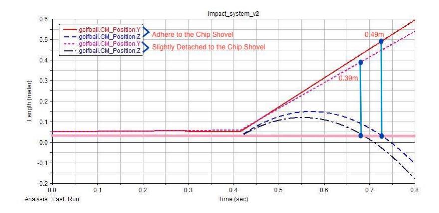
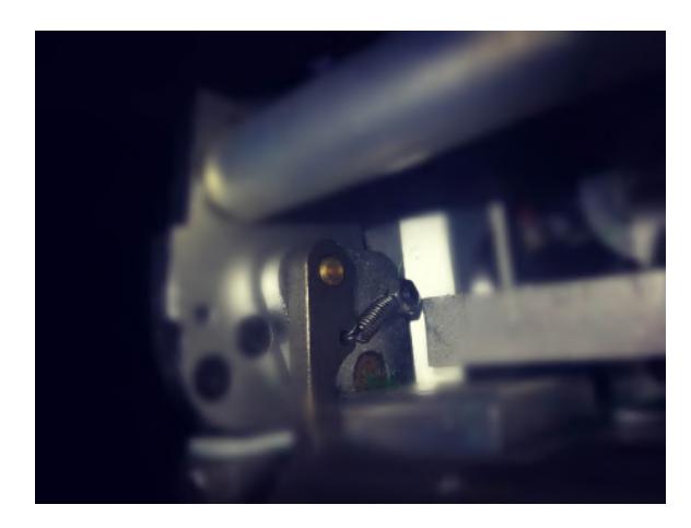
Add a tension spring to pick shovel to solve the shovel vibration caused by the problem of unsteady dribbling. Our study found that when the surface of the ball is close to the surface of the shovel, the kinetic energy delivered most efficiently and stably. Therefore, our team will launch the dribbling motor so the ball will be absorbed firmly in the shovel surface. Since we have no restriction on the direction of rotation of the shovel, it causes a large vibration when the ball is dribbled and the robot moves which affect the stability of the ball dribbling. As the result of ADAMS shows, adherent to the chip shovel or not while chip kicking, the distance that the ball can travel differs differently, with 0.49 meters (adherent) and 0.39 meters (slightly detached).
Improve Chip and Shot Stability
The conditions of flat-shot stability were studied and the linear bearing version was tested. Our strategy has high requirements on the stability of the pick-and-roll of the hardware, and we have studied various factors that influence the stability of the pick-and-roll. One of the most important factors is the frictional resistance. Due to the sliding friction between the iron core and the solenoid, the frictional force is uncontrollable, which will result in instability of the pick-up action. Therefore, we try to use a linear bearing to frame the core so that there is no contact with the solenoid. The friction on the linear bearings is rolling friction, which is small and stable, and the experimental data are also very stable, which also proves our conjecture. But the main problem at present is that the linear bearing occupies a lot of space. We have to reduce the number of turns of the solenoid and the diameter of the iron core, which caused a sharp drop in the maximum distance of the chip shots. Therefore, we will conduct the electromagnetic simulation of the solenoid and establish the impact model of the entire pick-up system to find the optimal solution to meet the demand of the pick-up distance in the future larger venues.

Solve Shovel Vibration tension spring result
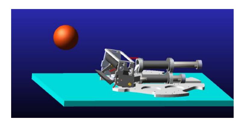
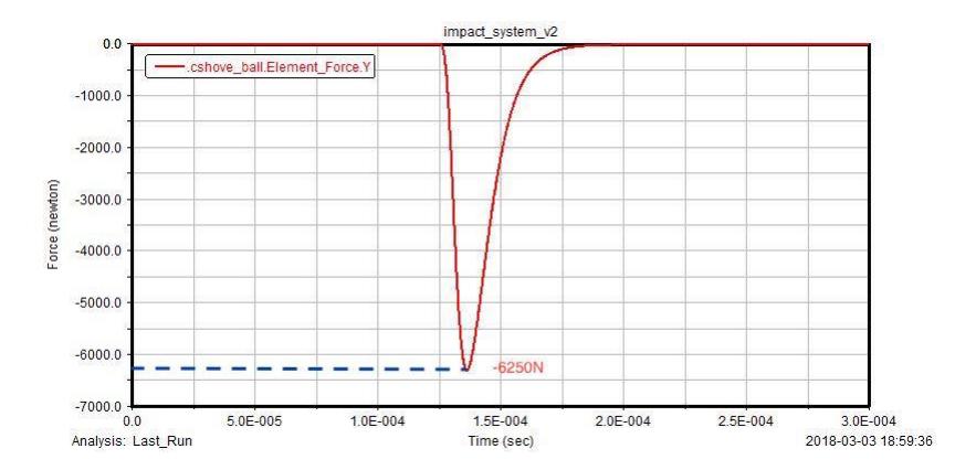
Therefore we added a tension spring to the newly designed shovel to restrain its vibration, and we do get good results. On the other hand, we verify that the tensile force of the tension spring is not an order of magnitude greater than the impact force of the pick. The impact force at which the shovel drives the ball only 1.5meters (which is far below the level of our actual combat) is shown in the figure below. Practically, adding the tension spring has no negative impact on the pick-up performance.
2.2 Electronics
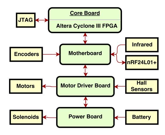
Since RoboCup 2011, the overall structure of the robot's electrical system shown in the Figure 9 below hasn't changed, though there were quite a lot effort on developing more advanced and integrated circuit boards. During the test period, the stability and maintainability are the primary concern. The adopted changes were integrating Brushless DC Motor Controller (ON Semiconductor MC33035) into FPGA and using separate motor driver boards containing gate drivers and MOSFETs for each motor. Higher movement performance and position precision of the robot is needed for future competition.
Improvements and ARM Controller
There are three major improvements made so far to enhance the robot's motion ability. First, we added an ARM MCU to take over tasks except for the motor control which is integrated into the FPGA. The saving logical gates are used for extra motor control features and encoder faulty detection. Second, since the number of robots will increase to 8 and further to 11, we redesigned our base station to allow higher communication rate with both the strategy computer and the robots. The communication protocol was also modified to carry the robot's position data and path plan information. And the last, a nineaxis motion processer unit was used to track the robot's position between vision frames, which increased the robot's localization and path following precision. Details are discussed below.
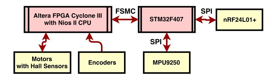
The STM32F407 MCU is now added to the core board to handle communication and robot configuration. The structure of controller are shown in the Figure 10 below. The FPGA is dedicated to motor control. The desired velocity of each motor is transferred by ARM MCU using flexible static memory controller (FSMC). After decoding wireless data package, the ARM MCU plans the S-Curve acceleration and deceleration of the motors based on the path information contained in the package. Acceleration constraints are applied during the velocity plan, which assures smooth and fast speed change of each motor.
Sensor Fusion
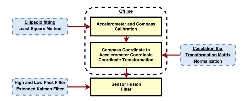
The MPU9250 sensor integrates gyroscope, accelerometer and compass. Though the Digital Motion Processor (DMP) developed by Invensense is integrated into the chip, which allows 6-axis sensor fusion calculations to be performed at a fixed rate of 200Hz. This capability is important for the primary application of this chip in the smart phone and tablet markets. For the usage in our robot, we implement sensor fusion algorithm which is transparent and easy to modify. The sensor fusion requires three steps in the Figure 11 below. First, each individual sensor requires calibration. Second, the coordinate transformation between the accelerometer and compass. Third, the sensor fusion and filter conducted using realtime calculation algorithms.
Base Station
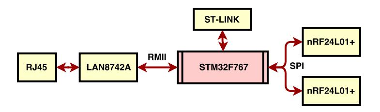
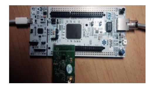
With more robots on the field, original wireless module using nRL2401A with 1Mbps maximum data rate is not enough for at least 60Hz update frequency on each robot. The original interface (USB to UART by CP2102, 1Mbps maximum baud rate) between the base station and strategy computer also requires upgrade. The hardware of new base station is outlined in the Figure 12 below. The design of base station refers to Team TIGERs Mannheim's open-sourced one. We are grateful for their contribution to other teams in Small Size League. Our demo base station is based on STM32F767 Nucleo-144 development board shown in the Figure 13 below. We will release the hardware design and embedded software of our base station later which only requires a low cost development board and nRF24L01+ modules.
Communication Protocol and Path Specification
New communication protocol contains planned path and current location information for the robot. We specify three types of path in the wireless package shown in the Table 1 below referred to numerical control in machine tools. The linear one contains the number and property of line segmentation. The circular one defines the property of the circle. The Bézier curve uses four control points, robot's current position, control point P1, P2 and the desired position.
Original communication protocol just specified the robot's desired velocity.
The position control loop was conducted on the strategy computer. With the added MCU, motion sensor and expansion in communication data rate, the position control loop is implemented in the robot.
Table 1. Planned Path Data
| Skill - Path Follow |
Linear | Circular | Bézier Curve |
|---|---|---|---|
| Skill Data | Number of Line | Desired Position and | Desired Position and |
| Segments | Orientation | Orientation | |
| Desired Position and | Desired Velocity at the | Desired Velocity at the | |
| Orientation | Destination | Destination | |
| Desired Velocity at the | Control Point P1 | ||
| Destination | |||
| Control Point P2 |
Software
3.1 Vision Module
The vision of the field is the most essential and reliable way to acquire all the information of robots and ball. Since a considerable change this year is that the field becomes larger and the number of cameras increases from four to eight, our team decides to gain more useful information from the vision via following ways.
Distortion Correction
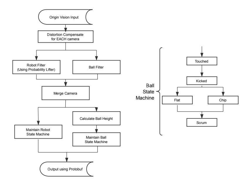
Since the distortion treatment on the vision-computer is not always perfect and the environment in hall varies from time to time, we find it essential to add a distortion compensation on vision so that we can fit the field better and filter only one ball on each frame once we receive the origin vision message. We are also able to calculate ball height via more cameras. When the same ball appears in more than one camera vision, we can figure out its height and thus determine if it's in "flying" status.
New Filter
We apply a brand-new robot position filter algorithm called Probability Lifter. When a robot appears in the camera vision we set a low confidence to it and slowly raise it when the robot stays in the vision. Vice versa, when a robot disappears from vision, we would slowly decrease the confidence instead of directly delete the robot position while processing data. This makes the robot filter more stable and handles the sudden disappearance of robot well.
Vision Filter for Ball
As for the ball filter, we also use the Probability Lifter above to make a more accurate and stable vision. What's more, in order to get necessary information for our strategy algorithm, we add the ball model to our filter and maintain a state machine based on the visual input. The state machine maintains whether the ball is kicked off by a robot or held by a robot. Using our collision detect algorithm, we can also detect the last robot touched (including kicked) the ball.
Therefore, we getting more beneficial information from the original vision and enable our decision module using more reliable data to make both effective and excellent decision.
3.2 Motion Control
Motion control is one of the most basic but essential sections in robots. Robots cannot conduct any kinds of actions without motion control section. On the one hand, the SSL has quite high velocity and acceleration on the field, compared to other leagues in RoboCup. Therefore, the robots on the field must have the ability to change their velocity and direction in very short time in which way they can intercept a rolling ball or avoid a collision. On the other hand, sometimes the specific time of robots conducting actions is needed. With a proper motion control model it can be obtained easily. Based on the above requests, we are planning on modifying our motion control system.
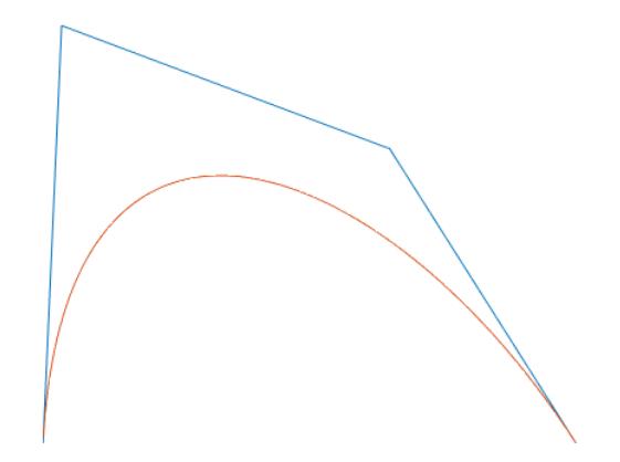
The first issue we considered about in this system was the planned path. It is supposed to be as smooth as possible so the robots won't bear a overwhelming acceleration which might cause a tumble. Previously, we would set several positions which the robots will go by. But now, in order to make the path more smooth, we decide to take advantage of the Bézier Curves.
Bézier Curve Path Planning
As the above figure shows, with the Bézier Curve, we can generate a smooth curve based on appropriate control factors. We can modify the velocity factor and distance factor to change the locations of control points, which then changes the shape of the curve. So we can set the appropriate factors to fit our robots best. While on the other hand, if a robot needs to avoid collision when it is moving, a new Bésier Curve will be generated. And the new curve will still begin with its current velocity and acceleration. In this way the robot can avoid a sudden change on its motion states and reduce the energe loss on the dodging process. We hope it could help our robots move more smoothly and decreace unneccessary collision.
Timed-Elastic-Bands Motion Control
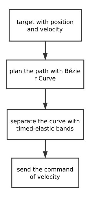
After the path is generated, the next issue is about how we can divide different stages and set the motion commands sending to the robots. The basic motion control algorithm we referred to is the Timed-Elastic-Bands. Before when we wanted a robot to move to a specific point, we would do a trapezoid planning with max acceleration and estimate the time spending on the road. But this time instead of that, we would firstly set the time in which the robot is supposed to be at that point. Next we divide the time into several parts with the frame in which we send control messages. With these sections of time, we can generate the control points in the Bésier Curve. The distribution of the control points will be more intensive in where the curvature is larger, indicating a lower velocity. Then the velocity and the corresponding acceleration will be examined in case they are beyond the constraints.
If, at the conducting process, there suddently burst a robot which need to be dodged, a new curve will be generated with the robot's current state as the initial control point. Besides, the motion parameters of the robot will be adjusted, such as increase the velocity, so that the robot can still arrive in time. Additionally, in this way the possibility would also be decreased where robots might tumble when its acceleration suddenly changes.
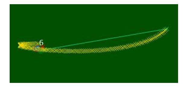
Benefits of Motion Control
As we can see in the figure, the acceleration is no longer a constant value, but can be adjusted by its motion posture in the moving process. In some stages the robot can keep uniform velocity and in others it will take its max acceleration to reach those specific states.
Therefore, with the Timed-Elastic-Bands and Bésier Curve, we could achieve the following benefits:
- Robots can have smooth moving process on the field.
- Robots can avoid collision more nimbly and with less risk of tumble.
- The robots' moving time can be obtained easily and precisely.
3.3 Parameters Self-Adaption Module
Parameters play an essential role in RoboCup court. For example, when sending a shooting signal to a robot, there is a parameter-based mathematical model between the coil's discharge time and actual outlet speed. When a robot receive a moving ball, there exist a relationship between the outlet angle and ball's velocity and injection angle. So in order to shoot precisely along a certain position, a rotation angle is needed. The parameters, which may change over time and vary from different court, are currently measured and fitted manually. In this paper, we propose a robust method to make the parameters self-adaptable based on what happened on the court, which not only enhances the automation of the robot soccer team but pave the wave for the future learning algorithms.
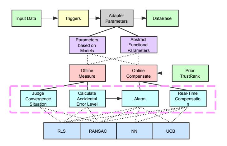
The overall process of this module can be derived from the chart below. The self adaption process begins after triggering, with both paramter based model and nonparametric model to solve a certain problem. In the measurement process, we have the methods of both off-line measuring and on-line measuring, while the former of which measure the overall situation of the model and the latter of which can adjust according to the online situation. The fourth and fifth rows of the chart show the concrete methodology of the system.
Models
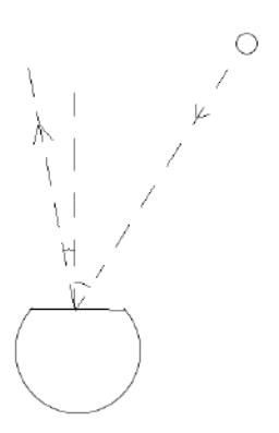
First thing to build the system is to establish a well-fitted mathematical model. Taking the compensation process as an example. As is shown in following figure, when a robot receive a moving ball, the outlet angle and ball's velocity and injection angle may satisfy the relationship: $\sin(\theta_{out}) = a \times v_{in} \sin(\theta_{in}) + b$. In order to shoot along a certain direction, direction A shown in figure below, a compensated angle is needed. According to the approximation that in small angle, $\sin(\theta) \approx \theta$, as well as some trival mathmatical derivation, we get the compensated angle $\theta = \frac{a \times v_{in} \sin(\theta_{in}) + b}{1 + a \times v_{in}}$
Measurement
Offline Measure. During offline measurement, in view of the outliers which occur frequently, we may use RANSAC instead of standard LS to fit the data. In the measured dataset, we firstly calculate the variance of the data and apply it to RANSAC algorithm.
Online Compensate. As the parameters vary with the changing situation on the court, for example, the mechanical structure of the vehicle changes due to collision, we also need to measure the parameters of the court on-line. The method can be RLS, whose cost function is $V = \sum_{n=1}^{N} \lambda^{(N-t)} (y(n) - \Phi^T(n)\hat{\theta})^2$. The forgetting factor $\lambda$ is often set at 0.95, which enable the latest data dominates the fitting while previous data still play a part. This guarantee the dynamic adaption of the parameters. When performing on-court measurement, we can use Bayesian Linear Fitting to correct the parameters online.
$$\text{initialize: } \Sigma_0^{-1} = \mathbf{0}, \Sigma_X = X_{initial}, \sigma_y = Y_{initial}$$
During every iterations, according to the measured data, do the following calculation iteratively.
$$\Sigma_i = \left(\widetilde{X}_i \sigma_d^{-1} \widetilde{X}i^T + \Sigma{i-1}^{-1}\right)^{-1}, \quad \bar{\mu}_i = \left(\widetilde{y}i \sigma_d^{-1} \widetilde{X}i^T + \bar{\mu}{i-1} \Sigma{i-1}^{-1}\right) \Sigma_i$$
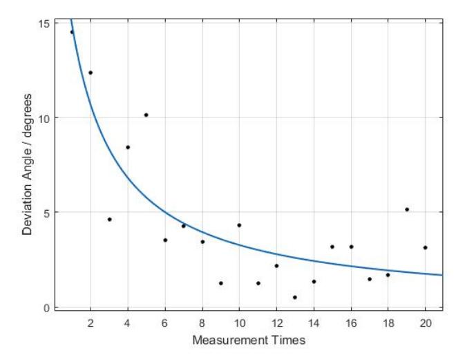
The result of the compensation can be seen from this figure. As time goes on, the deviation angle between actual outlet direction and expected direction becomes increasingly small overtime.
Self-Adaption
Judge Convergence Situation. During the measurement process, it is easy for us to get the variance of the known model. Considering the complicated situation that may occur on court and the possible outliers, the convergence criterion are made based on prior knowledge.
Alarm. Besides conducting online measurement and compensation, alarms are also sent when one robot certainly need to be carefully examined. When a measured data shows that the robot's performance is far from expected, then human intervention is needed to check the robot.
Real-Time Compensation. When conducting a certain task, apply the calculated compensation value into the system.
3.4 Passing in Normal Play
Situation Judgement Module
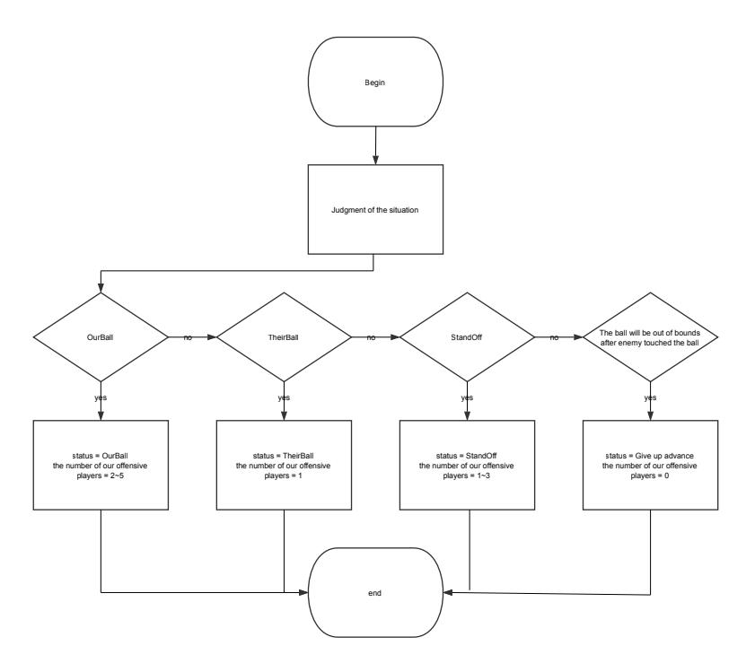
At the beginning of the module, we should determine the ownership of the ball, which can be divided into 4 states: our ball, others' ball, the ball standing off, the ball moving out of bounds. When the state is determined, start counting the number of offensive players needed. The number of offensive players is fixed when the ball is held by the opponent or will be out of bounds soon. The process can be seen from Figure 21. After this process, we can determine the number of the offensive players.
Offensive Value Calculation
After determining the number of offensive players, we turn to a modeled value to determine which robots should be the offensive one. The calculation of offensive players, termed Offensive Value, is divided into 3 parts. The first part is based on the location of the ball after we get the ball. The closer to the goal, the greater the value, which derive Offensive Value v¹ = α × dgoal. The second part is based on the success rate of passing, where the closest player, both in our team and the opponent's, from the player is taken into account. The Offensive Value is v² = β(−doutclosest + dtheirclosest). Finally is based on the Predictor Receiver. Finally, the various parts multiplied by the part of the weight and then add to get the final advantage value. According to the value of the dominant player , we determine the number of offensive players. In the state of confrontation, we give a threat value to each other, if the opponent can grab the ball faster than us, threat value gets relatively high. The module ends after determining the best offensive opponents.
Decision Module
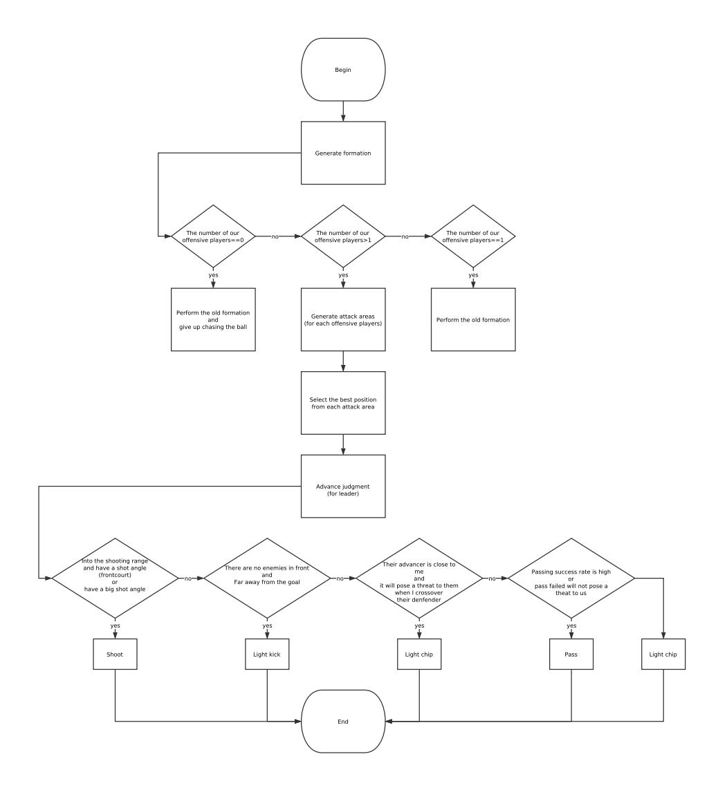
Decision Module aims at determine which play should be selected. In the beginning of the module, if we are not on the attacking process, simply switch from getball to protect shoot line, which are terms describing the decision to get a ball and to defend on the opponents' possible shooting line, respectively. If only one attacking player is needed, just use of the previous method to determine which play should be selected. If the attacking player number is greater than one, which is, there is at least one Receiver, so we began to generate the attacking area for Receiver1, and calculate the best receiving position. As for Receiver2, both the position of Leader and Receiver1 should be taken into account. When more Receiver is needed, simply consider the previous Receivers recursively and determine the best receiving position.
If a position where robots can shoot without dribbling, pick these points out and calculate the best shooting point in view of the distance and angle from the goal. Taking a step back, if no perfect shooting point is found, just pick the points where robots can first turn and then kick. If neither shooting points nor receiving points are found, just pick the closest point in the Receiver area from the goal.
After adapting to the new decision module in our system, both the offensive and defensive status are smoother and revieving a more successful effect, comparing to last year's efforts.
Conclusion
In this year, we are trying to develop new passing method in the NormalPlay. Besides, new motion control methods and parameter adapter is developed. This paper mainly discuss the big changes happened to our hardware designs. We are working in several ways to make our robots more stable and more aggressive. In next year, we will continue to focus on the multi-agent cooperation to make our strategy more intelligent.
References
- STmicroelectronics. STM32F407xx Datasheet, 2012. http://www.st.com/en/microcontrollers/stm32f4-series.html?querycriteria=productId=SS1577.
- Andre Ryll, Mark Geiger, Nicolai Ommer, Arne Sachtler, Lukas Magel. TIGERs Mannheim Extended Team Description for RoboCup 2016, 2016.
- STmicroelectronics. STM32 Nucleo-144 Development Board, 2017. http://www.st.com/en/evaluation-tools/nucleo-f767zi.html
- MICROCHIP. LAN8742A Datasheet, 2015.
- Tianyao Gao, Yanan Wu, Tong Yang, Zheyuan Huang and Rong Xiong. ZJUNlict Team Description for RoboCup 2017, 2017. http://wiki.robocup.org/images/b/bc/Robocupssl2017-final21.pdf
- Keller, Martin, Frank Hoffmann, Carsten Hass, Torsten Bertram, and Alois Seewald. "Planning of optimal collision avoidance trajectories with timed elastic bands." IFAC Proceedings Volumes 47, no. 3 (2014): 9822-9827
- Jolly, K. G., R. Sreerama Kumar, and R. Vijayakumar. "A Bezier curve based path planning in a multi-agent robot soccer system without violating the acceleration limits." Robotics and Autonomous Systems 57, no. 1 (2009): 23-33.