MCT Susano Logics 2019 Team Description

Koki Inoue, Naoki Kanyama, Shohei Degawa, Yuki Kurosaki, Toshiyuki Beppu

National Institute of Technology, Matsue College 14-4, Nishi-Ikuma, Matsue, Shimane, 690-8518, Japan

http://www.matsue-ct.ac.jp/

Abstract We developed algorithms for avoiding robots of the opposing team, since the SSL rules require each team to avert a robot crash. The algorithms are heuristic methods; team AI determines robots to avoid, calculates the tangent line to a collision range circle of the opposing team's robot from a team robot, sets the path line of team robot to the tangent line of an extended collision range circle of the opposing team's robot, and limits the robot speed for returning the robot direction to the target position after an avoidance. Keywords: RoboCup, SSL, obstacle avoidance, omnidirectional mobile robot.

1 Introduction

MCT Susano Logics was founded in 2011, and the team was named after a hero of Japanese mythology, Susano. Susano was a brother of Amaterasu, the goddess of the Sun. He exterminated a huge dragon Yamatano-Orochi which had an eight-forked head and an eight-forked tail. Our team was named with the hope of defeating strong and intelligent dragons in SSL.

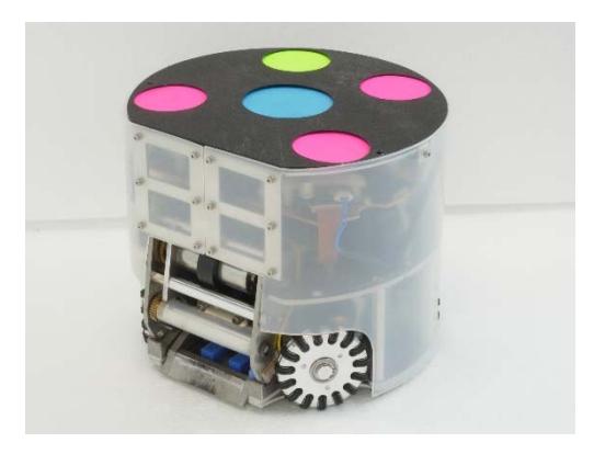
Susano Logics have been taking part in the RoboCup Japan Open since 2011 and in the international contest, RoboCup, since 2013 in Eindhoven, Netherlands. Our robots have a distinctive transparent shell (Fig. 1), however the specifications of robots and performance of AI are not at all outstanding. This year, we developed algorithms to avoid collision with our opponents, since the SSL rule requires each team to avert a robot crash. we improved our software. This TDP describes our algorithms.

2 Robot Control Methods

2.1 Low Level Controller of MCT Susano Logics' Robot

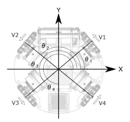
Figure 2 shows the bottom view of MCT Susano Logics' robot. The robot has four omni wheels of 50 millimeters in diameter. Each omni wheel has 15 small discs of 10 millimeters in diameter. The height of the robot is 143 millimeters, the weight is 2.5 kilograms and the height of the center of the gravity is 55 millimeters.

If the small discs revolve with no friction and there is no skid between the direction of wheel rotation angles and the floor, the wheel rotation speeds $V_1$ to $V_4$ are the components of the robot speed vector $V \angle \theta$ and the robot rotation speed $V_{\omega}$.

$$\begin{pmatrix} V_1 \ V_2 \ V_3 \ V_4 \end{pmatrix} = \frac{1}{r_{wheel}} \begin{pmatrix} -\frac{1}{\cos\theta_1} & \frac{1}{\sin\theta_1} & r \ -\frac{1}{\cos\theta_2} & -\frac{1}{\sin\theta_2} & r \ \frac{1}{\cos\theta_3} & -\frac{1}{\sin\theta_3} & r \ \frac{1}{\cos\theta_4} & \frac{1}{\sin\theta_4} & r \end{pmatrix} \begin{pmatrix} V \sin\theta \ V \cos\theta \ V_{\omega} \end{pmatrix}$$

where $\theta_1$ to $\theta_4$ are mounting angles of omni-wheels, which are 40, 140, 220, 320 degrees, $r_{wheel}$ is the radius of the omni-wheel.

We programmed Eq. (1) to our controller and tested it. The robot speed for lateral direction was accurate but for the longitudinal direction was about 24 per cent too low. We could not find the reason for the lowering of the speed. We devised an adjustment equation to compensate for robot speed experimentally. The compensated speed of the robot V' is,

$$V' = (1 \times 10^{-5}\theta + 3.05 \times 10^{-3} + 9.76 \times 10^{-1})V$$

The error between the robot speed and its command are within 4 per cent of the adjustment equation.

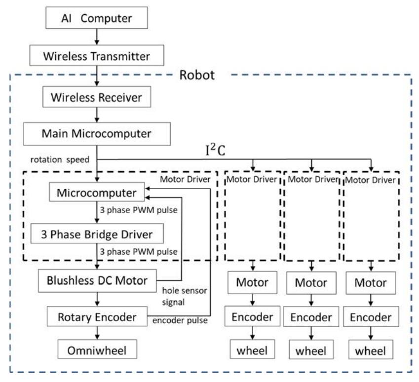
Figure 3 indicates the control system of MCT Susano Logics' robot. The control system consists of a main one-chip microcomputer (Microchip, dsPIC33FJ32GP202) and four motor drivers. The main microcomputer receives commands from team AI computer via IEEE 802.15.4 wireless communication module (Digi International, XBee S1) and calculates motor rotation speeds $V_1$ to $V_4$. The main microcomputer sends the rotation speeds to motor drives via I²C communication line.

The motor driver consists of a one-chip microcomputer (Microchip, dsPIC33FJ12MC202), a gate driver (Microchip, MCP14700), a three-phase H-bridge driver with six MOSFETs (Diodes Inc., DMG4822SSD), and a rotary encoder (US Digital, E8P). We adopted Maxon EC45 flat motors⁽¹⁾ and reduction gear of 35:80 ratio for driving the wheels. The EC45 motor has a built-in hole sensor to detect the rotor angle and to synchronize the PWM pulse to the angle. The sensor resolution of 48 pulses per round is not adequate for control at the minimum speed of 100 millimeters per second. We add a magnetic rotary encoder of 1440 pulses per round.

The microcomputer generates a three-phase PWM pulse at a control interval of 20 milliseconds. We adopt the torque/duty converter technique⁽²⁾ (Fig. 4). The PI controller calculates the output torque at time k, MT(k) from the desired angular velocity $\omega_{desired}$ and motor angular velocity $\omega(k)$.

$$\omega_e(k) = \omega_{desired} - \omega(k)$$

$$MT(k) = MT(k) + k_n \left(\omega_e(k) - \omega_e(k-1)\right) + k_i \cdot \omega_e(k)$$

Where $\omega_e(k)$ is the angular velocity error at time k, $k_p$ is the proportional gain and $k_i$ is the integral gain. Both gains are settled experimentally. The duty ratio of PWM pulse Duty(k) is,

$$Duty(k) = \frac{R}{K_m \cdot V_{cc}} \left( MT(k) + \frac{K_m}{K_n \cdot R} \omega(k) \right)$$

where $V_{cc}$ is the battery voltage (11.1 V), R is the motor coil resistance, $K_m$ is the motor torque constant, $K_n$ is the motor speed constant. These values are indicated in the data sheet.

Fig. 2. Bottom View of MCT Susano Logics' Robot

Fig. 3. Block diagram of Robot Controller

2.2 Robot Speed Control

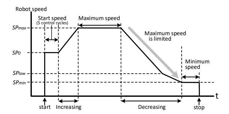
Figure 4 shows the speed control sequence of our robot. At the start, the AI sends a start speed value SP0 to robots. We normally set SP0 value to 1.2 meter per second, but decreased to 0.8 or 1.0 meter per second on slippery fields. The AI keeps the speed value constant during five control cycles of waiting for the acceleration of the robot. We set the maximum speed of the robot SPmax to 3.0 meters per second experimentally. When the robot approaches the target position, the AI limits SPmax from the distance between the robot and the target position for not to overpass the goal. When Dist_ob is larger than 60 millimeters, SPmax is,

$$SP_{max} = \sqrt{0.0048 \times Dist_{ob} - 0.22} - 0.26$$

If Dist_ob is less than 60 millimeters, the AI will keep the robot speed to the minimum value of SPmin. We set the SPmin to 0.01 meter per second.

The AI varies the robot speed at every control cycle of 16 milliseconds. We set the variance Δ to േ0.04 meter per second. When the robot speed becomes low, Δ is set to -0.02 meter per second, in order to keep the high speed. The robot speed at time k SP(k) is,

$$SP(k) = SP(k-1) + \Delta SP$$

$$\Delta SP = \begin{cases} +0.04 & |SP(k-1) < SP_{max} \ -0.04 & |SP(k-1) > SP_{max} \text{ and } SP(k-1) > SP_{low} \ -0.02 & |SP(k-1) > SP_{max} \text{ and } SP(k-1) \le SP_{low} \end{cases}$$

where SP_low is the threshold of Δ and we set the value to 0.03 meter per second.

Fig. 4. Speed Control Sequence of the Robot

3 Obstacle Avoidance

To find a robot path for avoiding opponent team robots, we once adopted a rapidly exploring random tree (RRT) algorithm. The RRT succeeded to find a path, however, quick movement of opponent team robots forced team AI to find another path in a short time. Furthermore, the RRT often found a new path on reverse direction, thus the robot came back and forth. Therefore, we abandoned this method.

3.1 Obstacle Avoidance Algorithms

DPL Coordinate System

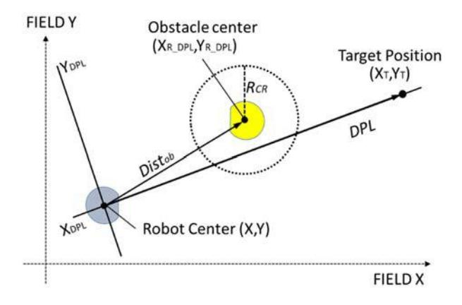
Figure 5 indicates the basic idea of a desired path line (DPL) coordinate system⁽³⁾. Assuming a robot on the real field wants to reach the target position, a line drawn from the robot center (X, Y) to the target position (X_T, Y_T) is DPL. We introduce a relative coordinate system with the robot center as the origin and the DPL as the x-axis. On DPL coordinate system, the target positon (X_{T_DPL}, Y_{T_DPL}) is on the DPL x-axis thus,

$$(X_{T_{DPL}}, Y_{T_{DPL}}) = (\sqrt{(X - X_{T})^{2} + (Y - Y_{T})^{2}}, 0)$$

The x coordinate of the target position X_{T_DPL} shows the distance from the robot to the goal.

Distance is the distance from the robot to a robot of opposing team (obstacle) (X_{R_DPL}, Y_{R_DPL}) is,

$$Dist_{ob} = \sqrt{X_{R_{_}DPL}^2 + Y_{R_{_}DPL}^2}$$

A circle around an obstacle with a radius of twice the radius of SSL robots R_CR indicates the collision range. If the DPL intersects the circle R_CR, the robot will collide with the obstacle. We allow a margin of 70 millimeters thus set R_CR to 250 millimeters, because we use the radius R_CR to judge start avoidance.

Fig. 5. Basic Idea of DPL coordinate system

Single Obstacle Avoidance

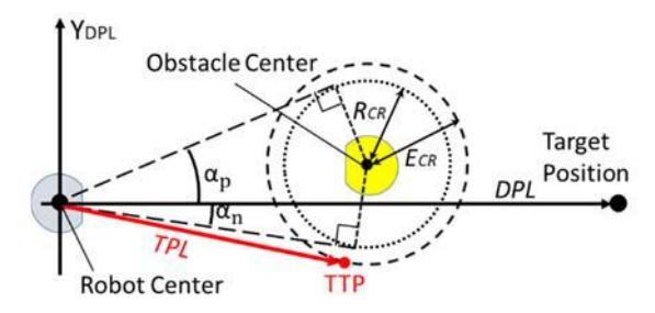
Figure 6 shows the temporal target position (TTP) calculated on DPL coordinate system. If the circle R_CR intersect the x-axis, AI calculates angles between the x-axis and the tangent lines from the circle R_CR to the robot center.

Assume angle θ_1 is the angle between the line from the center of obstacle to the origin and the tangent line from the circle R_CR to the origin. Angle θ_2 is the angle between the line from the center of the circle R_CR to the origin and the x-axis.

$$\theta_1 = \sin^{-1}\left(\frac{R_{CR}}{Dist_{ob}}\right)$$

$$\theta_2 = \tan^{-1} \left( \frac{Y_{R_DPL}}{X_{R_DPL}} \right)$$

The angle in the first quadrant α_p and the fourth quadrant α_n are,

$$\alpha_p = \theta_1 - \theta_2$$

$$\alpha_n = \theta_1 + \theta_2$$

Team AI selects the avoidance direction with the smaller value of $\alpha_p$ or $\alpha_n$.

We introduced an expanded obstacle circle with a radius of $E_{CR}$ in order to set a TTP and to find the position to end the avoidance. The coordinates of TTP are the contact point of the circle $E_{CR}$ from the origin.

$$(X_{TTP_DPL}, Y_{TTP_DPL}) = \begin{cases} (Dist_{ob} \cdot \cos(\theta_1) \cdot \cos \alpha_p, Dist_{ob} \cdot \cos(\theta_1) \cdot \sin \alpha_p) \ (Dist_{ob} \cdot \cos(\theta_1) \cdot \cos \alpha_n, -Dist_{ob} \cdot \cos(\theta_1) \cdot \sin \alpha_n) \end{cases}$$

The temporal path line (TPL) is also indicated on Fig. 6. We set the radius of $E_{CR}$ to 300 millimeters.

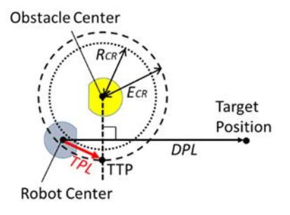
Sometimes the robot enters the circle $E_{CR}$. At that moment, team AI adjusts the TTP on the circumference of circle $E_{CR}$ (Fig. 7).

$$(X_{TTP_DPL}, Y_{TTP_DPL}) = \begin{cases} (X_{R_DPL}, Y_{R_DPL} + E_{CR}) & |\text{at } \alpha_p \text{ selected} \ (X_{R_DPL}, Y_{R_DPL} - E_{CR}) & |\text{at } \alpha_n \text{ selected} \end{cases}$$

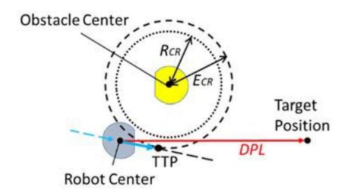
At the moment of the circle R_CR leaves the x-axis, team AI sets back the robot direction to the x-axis, DPL (Fig. 8).

As already mentioned in Eq. (6), we limit the moving speed of the robot by the distance between the robot and the target point (X_{T_DPL}). This is because if the maximum speed of the robot SPmax is limited by the distance between the robot and the TTP, our robot will arrive at the TTP with its minimum speed and will take too much time to reach the final destination. However, our robot cannot change direction at high speed at the end of the obstacle avoidance sequence.

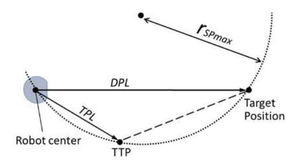
We assume a triangle of DPL, TPL and the line between the TTP and the target position and assume the circumscribed circle of the triangle (Fig. 9). Then we consider the radius of the circle rSPmax as the minimum turning radius.

The minimum turning radius of our robot with varying the moving speed SP were measured experimentally.

$$R_{min} = 262.5SP^2 + 252.5SP + 95$$

Therefore the SPmax from rSPmax is,

$$SP_{max} = \frac{-7.8 + \sqrt{R_{SPmax} - 34.28}}{16.2}$$

Fig. 6. Decision for the Temporal Target Position (TTP)

Fig. 7. Temporal Target Position for the Robot inside the Circle $E_{CR}$

Fig. 8. Returning from the Avoidance Sequence

Fig. 9. Decision Method for the Minimum Turning Radius

Multiple Obstacle Avoidance

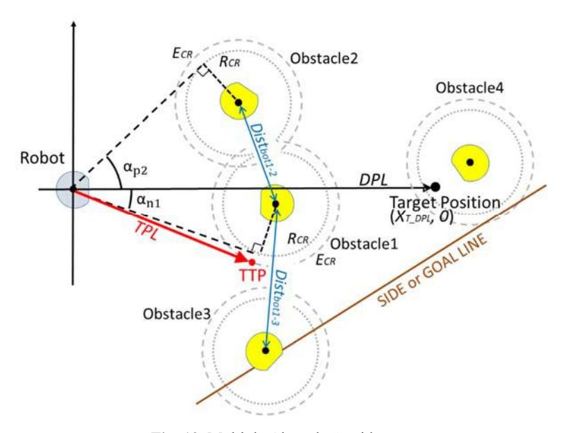
Figure 10 indicates the algorithms of multiple obstacle avoidance. If a circle R_CR of an obstacle intersects the DPL, team AI calculates the distance between the obstacle of intersected and all other obstacles (e.g. Distbot1-2). If the distance Distbot is too small to pass the robot (e.g. Distbot1-2), then AI checks the next obstacle. If Distbot is adequate for passing through (e.g. Distbot1-3) or no obstacle is next to the obstacle (e.g. left side of Obstacle 2), AI calculates and compares angle α_p and α_n for selecting the direction for avoidance. At the same moment, AI also checks the distance from the side or goal line of the field to the obstacles. If the extended circle E_CR of the obstacle intersects the side or goal line, AI selects another direction for the avoidance. In Fig.10, Distbot1-3 is wide enough and the circle R_CR of Obstacle 1 has no intersection point with the line, AI sets the TTP on the circle R_CR of Obstacle 1. Team AI is programmed not to check the obstacles which are further than the target point (e.g. Obstacle 4). We set the threshold width of passing through to 500 millimeters.

Penalty Area Avoidance

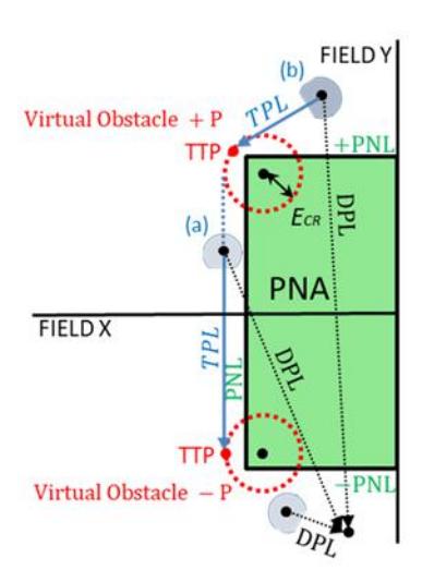
Figure 11 indicates the algorithms of the penalty area (PNA) avoidance. We set two virtual obstacles, +P and –P, which are (100, േ100) inside of the corners of the PNA. If the DPL of robot intersects the front line (PNL) and a side line (േPNL) of PNA (e.g. robot (a)), team AI sets the TTP on the circle R_CR of the virtual obstacle which is close to the side line of intersected (-P).

If the DPL of the robot intersects with both േPNL (e.g. robot (b)), team AI sets the TTP on the circle R_CR of the virtual obstacle of close to the robot (+P). If the robot (b) reaches to the circle of the virtual obstacle +P, DPL will not intersect +PNL.

Fig. 11. Algorithms of the Penalty Area (PNA) Avoidance

3.2 Experimental Results

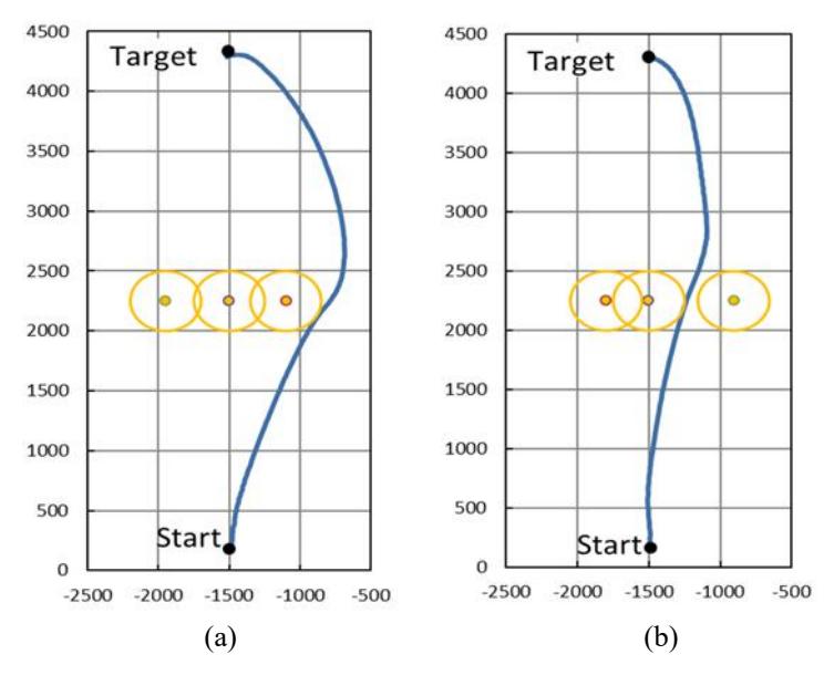
Figure 12 demonstrates two experimental results of obstacle avoidance. The blue line shows the trace of the robot, yellow dots show the center and yellow circles show the radius R_CR of the obstacles. The robot started from (-1500, 200) and ran to (-4500, 4300). There were three obstacles on y = 2250. In Fig. 12 (a) the robot went to the right side because there were not adequate spaces between obstacles, but in (b) the robot went through the obstacles. In both cases, the robot went too far from the obstacles and the recovery from the avoidance was not good. It might because of the excessive speed of the robot.

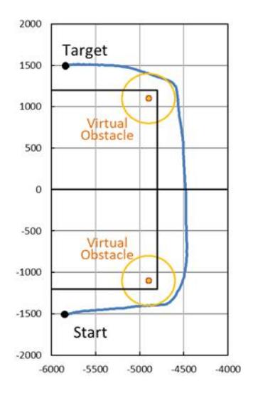
Figure 13 demonstrates robot trace of the penalty area avoidance. The starting position of the robot was (-5800, -1500). At the start position, DPL intersects both side lines of the penalty area, thus the robot went to TTL on circle R_CR of a virtual obstacle at (-4900, -1100). Then the robot turned around the circle of the virtual obstacle and went to TTL on another circle of the virtual obstacle. After passing through the second virtual obstacle, the robot reached the target position of (-5800, +1500).

Fig. 12. Results of the obstacle avoidance

Fig. 13. Results of the penalty area avoidance

4 Discussion

Our algorithms showed avoidance ability for static obstacles, however, robots of the opposing team move quickly and change direction often on the SSL field. We have to assess our algorithms in the context of a live game.

If both our team and opposing team's robots are running toward the same target position, they may crash. In this case, we should limit the robot speed strictly. However, if the target is the ball, it is important to arrive fast. We need to install sophisticated algorithms for judging the current situation.

References

Maxon Motor, EC45 flat. https://www.maxonjapan.co.jp/medias/sys_master/root/8830904893470/2018EN-265.pdf
K. Chaiso, K. Sukvichai. Skuba 2011 Extended Team Description. http://wiki.robocup.org/images/4/4c/Small_Size_League_-_RoboCup_2011_-_ETDP_Skuba.pdf
R. Williams II, J. Wu. Dynamic Obstacle Avoidance for an Omnidirectional Mobile Robot. http://downloads.hindawi.com/journals/jr/2010/901365.pdf