NAMeC - Team Description Paper Small Size League RoboCup 2019 Application of Qualification in Division B

J. Allali, J. Bezamat, A. Boussicault, R. Denieport, P. Felix, O. Ly, S. Loty, S. N'Guyen, V. Mignot, G. Passault, T. Saliba

LaBRI, Université de Bordeaux, France; ENSEIRB-MATMECA, Bordeaux-INP, France; CATIE, France; Bordeaux Ynov Campus, France

Abstract This paper presents some progresses of the NAMeC team since 2018. It includes changes in motor control, odometry, mechanics and electronics. For motor control we implement a field oriented control. For odometry we use a simple filter to aggregate vision and robot data. For mechanics we improve the dribblers, and for electronics we develop new boards.

1 Introduction

In 2018 we participated for the first time at the RoboCup SSL (division B) under the name AMC[7] (Aquitaine Mechatronics Club) that we had to change to NAMeC (Nouvelle-Aquitaine Mechatronics Club).

Unlike most of the teams – initially for mechanical reasons – we decided to design a direct drive wheeled robot (i.e. without gear reduction). Using more powerful motors (Maxon EC45 70W), the results were promising and we decided to stick to this principle. The main problem encountered was the lack of torque at very low speed, which is now solved by implementing a Field Oriented Control (FOC) mechanism. Moreover we also implemented an odometry that we lacked last year for a more precise position control.

Finally, we improved the dribbler and kicker mechanics in order to better control the pass behavior which was very difficult for us last year.

2 Software

(Section container)

2.1 Motor control with a field-oriented control

In our robot architecture, the propulsion is supported by brushless motors (MAXON EC45 24V/70W) in direct drive. We chose this method to save space and to avoid the hassle of making gearboxes.

Last year we used the internal hall sensors to detect the position of the magnets of the rotor. The phases of the motor was driven with six unique threebit codes provided by the three sensors.

As the motors are in direct drive, this method gives bad results at low speed (< 1.0 revolutions per second). Indeed, the rotor jumps from pole to pole and the movement has discrete position.

A better solution is to control the motor with a field-oriented control (FOC).

This method is pretty standard and our implementation is based on the application notes [2].

We successfully tested this control without current sensor, using only the magnetic absolute rotor position. This method is described below. Moreover, our new electronics is equipped with a current sensor in order to make this control even more precise.

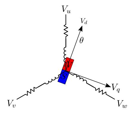
The idea of the method is to convert the three phase voltages/currents in two orthogonal voltages/currents phases expressed in the frame of the stator by using a Park transformation.

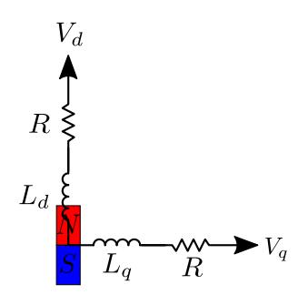
The figure 1 shows the three phases of the stator with the equivalent magnet of the rotor. The figure 2 shows the Park model of the system of the figure 1.

In the Park model, the Laplace equation of the system is :

$$\begin{pmatrix} V_d \ V_q \end{pmatrix} = \begin{pmatrix} R + sL_d(s) & -\omega L_q(s) \ \omega L_d(s) & R + sL_q(s) \end{pmatrix} \begin{pmatrix} i_d \ i_q \end{pmatrix} + \begin{pmatrix} 0 \ \omega \psi_a \end{pmatrix}$$

where

$$L_d(s) = L_d - \frac{M_{kd}^2 s}{R_{kd} + L_{kd} s}$$

and

$$L_q(s) = L_q - \frac{M_{kq}^2 s}{R_{kq} + L_{kq} s}$$

with the following Park transformation

$$\begin{pmatrix} V_d \ V_q \end{pmatrix} = \sqrt{\frac{2}{3}} \begin{pmatrix} \cos \theta & \cos(\theta - \frac{2\pi}{3}) & \cos(\theta + \frac{2\pi}{3}) \ -\sin \theta - \sin(\theta - \frac{2\pi}{3}) - \sin(\theta + \frac{2\pi}{3}) \end{pmatrix} \begin{pmatrix} V_u \ V_v \ V_w \end{pmatrix}$$

In those equations, Ld, Lq, Lkd, Lkq are inductances, Mkd and Mkq are mutual inductances, R, Rkd and Rkq are resistances. For more details, see the thesis of Afsharnia S. [6], page 54.

For our purpose, we use a simplified model where Ld(s) ≈ Ld and Lq(s) ≈ Lq are constant.

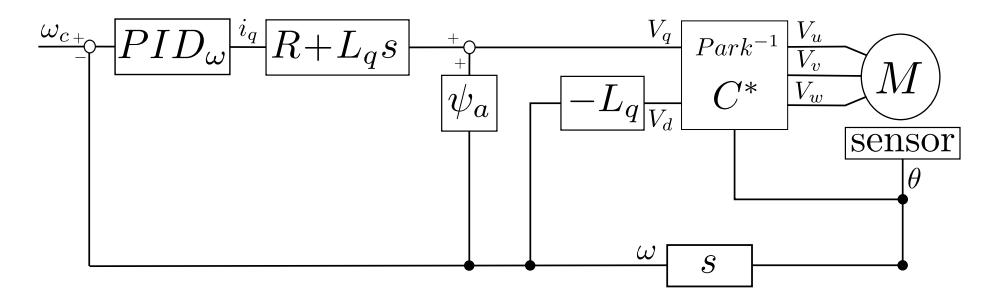
The field that is colinear to the magnet does not produce any torque on the rotor. The field that is orthogonal to the magnet produces the wanted torque of the motor. To determine the voltage of each phases, we just have to set id = 0 and iq to the value of the wanted torque.

Those remarks and equations gives the control diagram of Figure 3.

This architecture has been successfully tested by setting Lq ≈ 0 and for relatively low speed (greater that 0.4 revolutions per second and lesser that 11 revolutions per second). For even lower speeds, it is becoming difficult to actually measure the velocity.

However, we solved this problem for very low speed by controlling the motor with FOC by using the diagram (Fig. 3) in open loop. When we switch the control in low speed mode, we compute the desired angular position and apply the Park transformation with that angle by setting Vd to the maximal value possible (depending of the current we want to use) and Vq to 0. The drawback is that this open loop method is less power efficient (200 mA by motor instead of 40 mA with the closed loop).

We think our architecture can be used to obtain a speed greater than 11 revolutions per second. We don't check that hypothesis. Indeed, our magnetic rotary encoder (AS5048A) samples the angular position at 11kHz. In our current implementation, we imposed the following constraint :

$$\frac{\text{sample frequency}}{\text{Shannon factor} \times \text{sub sample rate}} > \text{motor velocity} \times \text{nb of pole pairs}$$

to be sure to have a correct control.

In our tests, the sample frequency was equal to 8kHz, the sub sample rate was equal to 10, the Shannon factor was equal to 10 and the number of pole pairs was equal to 8. From Equation 1, we deduce that the motor speed is limited to 10 revolutions per second. In practice, we obtain a limit of 11 revolutions per second.

To test higher speeds, we need to change the rotary encoder, and probably, we should set Lq ≠ 0.

Fig. 1. The three phases of a Brushless motor

Fig. 2. The Park model of a Brushless motor

Fig. 3. The control diagram of our motors

2.2 Odometry

Last year, the robots' motion control only relied upon the vision system. This was a limitation that made the control difficult. To solve this problem we want to integrate the vision information with the computation of the robot's odometry using wheels position sensors.

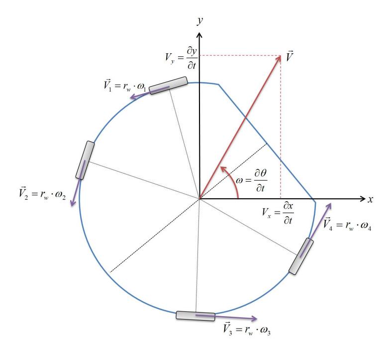
To do so, we need to compute the inverse kinematic model of the robot. This model gives the displacement of the robot (x, y, θ) knowing the displacement of each wheel. As the robots have four wheels, the matrix obtained is not square. The method used to obtain that matrix thus consists in computing the forward kinematic model (displacement of each wheel knowing the displacement of the robot), and then, to invert it using the least squares approximation (see Figure 4).

$$\begin{pmatrix} \partial tx \ \partial ty \ \partial t\theta \end{pmatrix} = A^{-1}_{4 \times 3} \cdot \begin{pmatrix} \partial tw_1 \ \partial tw_2 \ \partial tw_3 \ \partial tw_4 \end{pmatrix}$$

The matrix A⁻¹ is the Generalized Inverse of the matrix A computing the displacement of the wheels knowing the displacement of the robot. The Generalized Inverse is obtained with the following equation :

$$A^{-1} = A^T \cdot (A \cdot A^T)^{-1}$$

where AT is the transposed matrix of A

This common method is detailed in article [1].

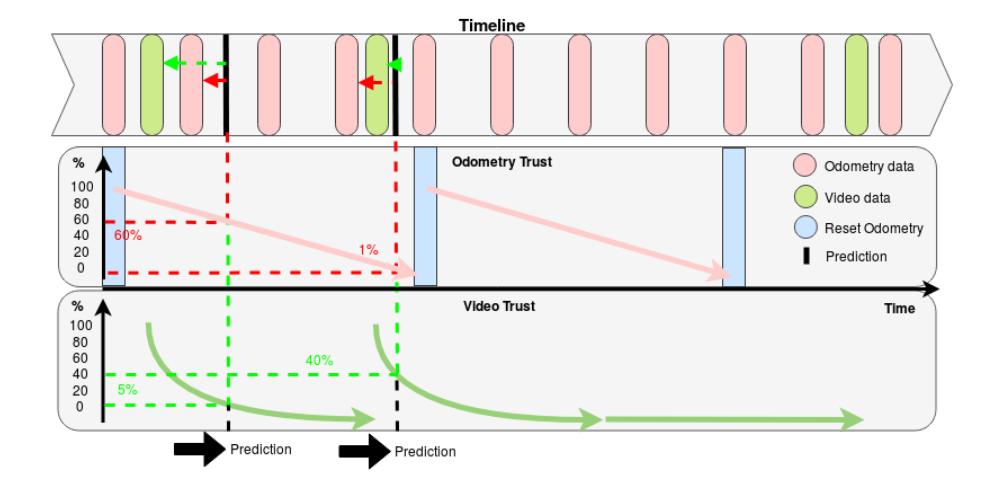
Then, odometry information have to be integrated with vision information. We implemented a simple filter (see Figure 5) giving a position prediction following the equation 4.

$$P(t) = \frac{p_{odom}}{p_{odom} + p_{video}} \cdot O(t_{last}) + \frac{p_{video}}{p_{odom} + p_{video}} \cdot V(t_{last})$$

P(t) is the prediction of the position and podom and pvideo are the trust factors of the data O(tlast) and V (tlast). This solution is not ideal but that way, the computer that leads the robots will be able to predict their positions for a short time even without vision or robot information.

This new solution has yet to be evaluated.

Fig. 4. Model used to compute the direct kinematic model.

Fig. 5. Idea of the implemented filter. Evolution of the $P_{odom}$ (percentage given by the red dashed lines) and $P_{video}$ (percentage given by the green dashed lines) according to the trust laws (respectively solid pink and solid green). The odometry trust is reset at a predefined frequency while the video trust is reset at each data reception.

2.3 Software architecture for the game strategies

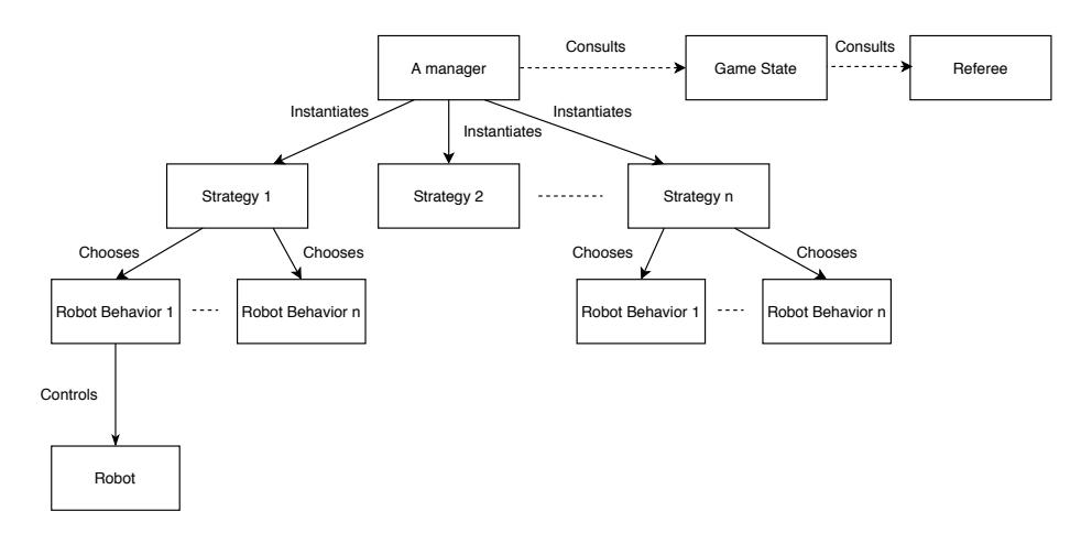
We implemented a new software architecture to manage our robots. This architecture was designed to allow developers to work independently on each part of the code (cf. Fig 6).

A state machine is created in GameState to organize the information sent by the Referee. This state machine is consulted by the Manager to prepare the robots for each phase of the game. In this architecture, the Manager have a general view of the match. It chooses the strategies to apply according to the situation and he assigns robots to the strategies. A Strategy is a simple coordination of a small number of robots to organize a specific attack or defense. The strategies assign behaviors to their robots. A robot Behavior is a basic action for a robot. For example, blocking an opponent robot, shooting the ball, clearing the ball in the opposing side.

Actually we have only one basic strategy. This strategy is reduced to a list of robot behaviors. We assign the robot behavior according to the number of available robots using that list.

Robot behaviors are also basic. The behavior that blocks the opposing robots, follows the middle of the segment connecting the ball to the opposing robot. The shooting behavior rushes the ball and shots as soon as possible. The wall behavior moves a robot in front of the ball and blocks all the shots at the goal. The goalkeeper behavior tries to predict the position of the ball (by integrating the linear speed of the ball) and tries to intercept the ball to avoid any goal.

Fig. 6. Schematic view of the software architecture for the strategies

2.4 Obstacle avoidance algorithm

The method we use is based on potential fields and aims at producing smooth trajectories. For each robot we compute impacts with each object o and the corresponding time to impact. If an impact is detected, the robot's position control is disabled and the obstacle avoidance is activated (based on velocity control). We implemented the method described in M. Mouad et al. (2012)[3]. This algorithm consists in computing the velocity vector of the robot by using a vector field defined by :

$$\begin{cases} \partial_t x = y + x \cdot (R^2 - x^2 - y^2) \ \partial_t y = -x + y \cdot (R^2 - x^2 - y^2), \end{cases}$$

in the relative frame of the obstacle.

This vector field forces the robot to turn around obstacles following a circular trajectory of variable radius R. The radius R being adapted to the situation (i.e. the value is different for the ball or for a robot).

For example, to reach the ball for a shoot, we use two phases:

1. we reduce R at the minimum value for the enemy and move the robot to the shooting position by avoiding the ball and the robots.
1. when we are close to the ball, we go to the ball and shoot without obstacle avoidance.

3 Hardware

(Section container)

3.1 Mechanics

Based on our experience from the RoboCup 2018 we decided to redesign our dribbler mechanism. Thanks to the advice and the open source design of the TIGERS Mannheim[5], we added some degrees of freedom and elastic dampers on the support of the dribbler in order to better control the ball and absorb impact shocks.

We also redesigned the coils and the chip kicker in order to make it more rigid and avoid the breaking problems we had in 2018.

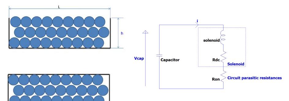
Since the goal of the kicker solenoid is to generate a strong magnetic field, we have tried to optimize the coil. The cross section of the coil is given figure 7

Assuming the diameter of the wire is d and the diameter of the wire is negligible compared to the length L of the solenoid, the number of turn per layer is $n_t = L/d$ . As wires have a round shape, $n_l = \frac{h\sqrt{2}}{d}$ .

Let be $l_e$ the average turn length. It is possible to compute the DC resistance of the winding : $R_{DC} = \rho \frac{l_e n_t n_l}{S}$ .

With S the section of the wire, thus $S=\pi\frac{d^2}{4}$ . We have $R_{DC}=4\rho\frac{l_eLh\sqrt{2}}{\pi d^4}$ . If the variation on the self-inductance is neglected, the magnetic field generation ated by the coil is proportional to the H-field : $B \propto H = n_t n_l i$ .

But, since the coil is voltage driven by a capacitor C initially charged at $V_{max}$ volts, and assuming a total parasitic resistance of $R_{on}$ (MOSFET's $Rds_{on}$ , interconnection, ...), this leads to (cf. Figure 8):

$$i(t) = \frac{V_{cap}(t)}{R_{DC} + R_{on}}$$

$$V_{cap}(t) = V_{max} \exp\left(-\frac{t_{kick}}{C(R_{DC} + R_{on})}\right)$$

According to [4], the energy transferred is proportional to the integral of the square of the current over time. Since we use two $2200\mu F$ capacitors charged at 180V:

$$E \propto \int_0^{t_{kick}} i^2(t) dt = \frac{1}{2} \frac{CV_{max}^2}{R_{DC} + R_{on}} \left( 1 - \exp\left(-2 \frac{t_{kick}}{C(R_{DC} + R_{on})}\right) \right)$$

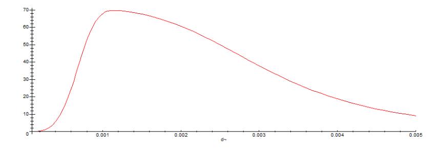
With the coil dimensions, the optimum wire diameter is around 1.2mm (see figure 9), with $L=5cm,,h=1cm,,l_e=6cm,,\rho=17.10^{-9}\varOmega/m,,t_{kick}=6ms$ and $R_{on}=10m\Omega.$

This is only a rough analysis to get the order of magnitude of the optimum coil wire diameter. We are currently testing different coil design, to validate (or not) this very simplified model.

Fig. 7. Cross section of the kicker coil

Fig. 9. Energy transferred (arbitrary scale) versus wire diameter(m)

3.2 Electronics

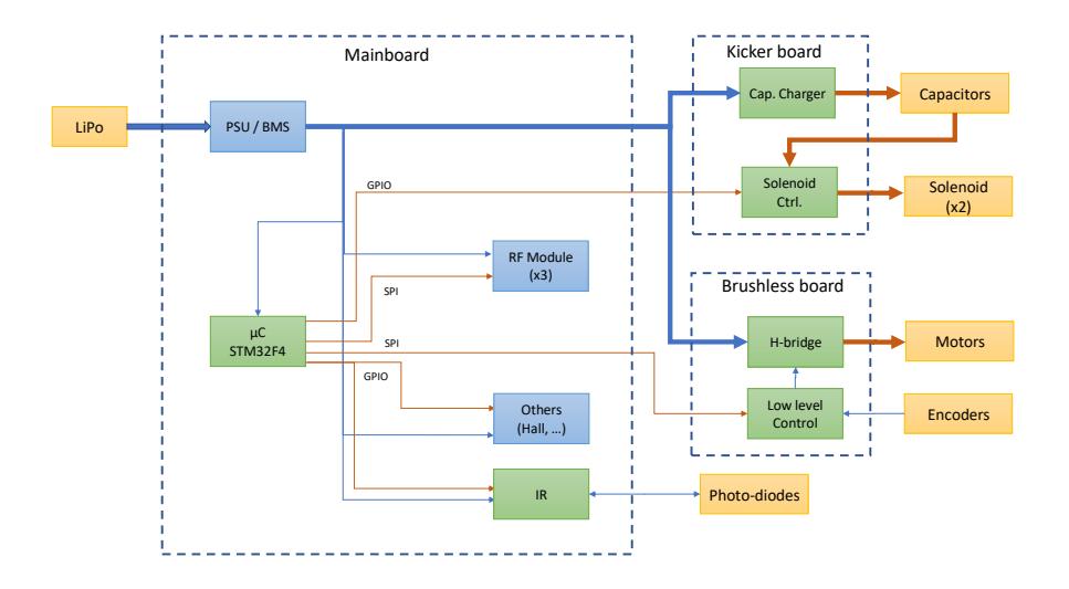
From the electronics point of view, the robot architecture is shown on the figure 10. A particular emphasis was made on modularity. Electronics boards are still in development, this is an overview of the main features.

The mainboard is based on a STM32F4 core that receives the orders from the master computer and dispatches them to all the other boards. Since the radio-modules use the very crowded 2.4GHz ISM band, a triple redundancy is implemented, each radio-module using a different channel, insuring that the data/orders are correctly transmitted even in a noisy environment.

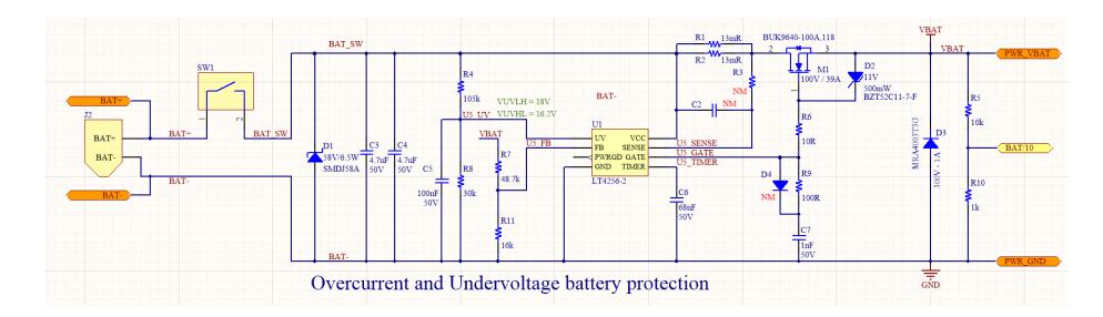
The mainboard also integrates a BMS (Battery Management System), which acts as an electronic (and smart) circuit breaker based on Linear Technology LT4256-2 circuit (figure 11). For safety reasons, if the current drawn by the robot is too high for too long, the BMS will cut of the power supply, thus preventing battery damage. It also checks the state of charge of the battery.

The brushless boards are used to drive each motor, their purpose is to insure a proper drive of all the wheels. There are in charge of the low level servo control, especially a FOC (Field Oriented Control) servo-loop control.

The kicker board stores energy into capacitors, and release it into the kickers solenoid. It is split into two parts:

Capacitor charger, based on a SEPIC converter. This DC/DC converter has the unique property to deliver a fixed power, when driven in discontinuous conduction mode. Since the power drawn is constant, this will not stress the battery when the capacitors are charged.
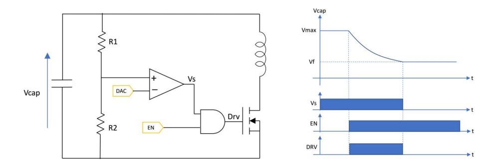
Solenoids driver. We will try to control the amont of energy fed into the solenoid to better control the kick power. This will be done by controlling the capacitor discharge voltage (figure 12).

The discharge threshold $V_f$ voltage is controlled by a DAC output and $V_f = 1 + \frac{R_2}{R_1} DAC$ . As long as the capacitor voltage $(V_{cap})$ is higher than $V_f$ and if the EN output is high, the MOSFET is closed. Assuming the capacitor is initially charged at $V_{max}$ , and discharged to $V_f$ , the amont of energy E transferred to the solenoid is $E = \frac{1}{2}C(V_{max}^2 - V_f^2)$ .

Fig. 10. Electronic architecture of the robot

References

Oliveira, Hélder P. Oliviera, Armando Sousa, António Paulo Moreira, Paulo J. Costa : Dynamical Models for Omni-directional Robots with 3 and 4 Wheels. ICINCO 2008 Proceedings of the 5th International Conference on Informatics in Control, Automation and Robotics.(2008)
RENESAS : Motor Control Application Vector Control for Permanent Magnet Synchronous Motor with Encoder (Algorithm). Applicatation Note R01AN3789EJ0101, Rev.1.01, (July 07 2017)
Mouad M., Adouane L., Khadraoui D., Martinet P. : Mobile Robot Navigation and Obstacles Avoidance based on Planning and Re-Planning Algorithm. 10th International IFAC Symposium on Robot Control (SYROCO'12), (2012), Dubrovnik, Croatia.
Paul H. Schimpf: A Detailed Explanation of Solenoid Force, Int. J. on Recent Trends in Engineering and Technology, Vol. 8, No. 2, Jan 2013.
Ryll A., Geiger M., Carstensen C., Ommer N. : TIGERs Mannheim: Extended Team Description for RoboCup 2018 RoboCup 2018, Montreal, Canada.
Afsharnia S. : Contrôle vectoriel des machines synchrones à aimants permanents : identification des paramètres et minimisation des ondulations de couple. Doctoral thesis supervised by Sargos, Franois-Michel supported at Génie électrique Vandoeuvre-les-Nancy, France (1995)
Boussicault A., Felix P., Hofer L., Ly O., N'Guyen S., Passault G., Pirrone A. : AMC - Team Description Paper, Small Size League RoboCup 2018, Application of Qualifcation in Division B, (2018)