NEUIslanders Team Description Paper RoboCup 2019

Prof. Dr. Rahib H. ABIYEV, Dr. Pavel MAKAROV, Ahmet CAGMAN, Ersin AYTAC, Gokhan BURGE, Ali TURK, Nurullah AKKAYA, Tolga YIRTICI, Gorkem SAY, Berk YILMAZ

NEU Robotics Lab. Department of Computer Engineering, Department of Electrical and Electronics Engineering, Department of Mechanical Engineering Near East University (NEU), Lefkosa, TRNC

http://robotics.neu.edu.tr

Abstract NEUIslanders team participates at RoboCup Small Size League since 2012-present. Last year in Montreal, Canada became SSL Division B champion. In this paper, it is explained in details how NEUIslanders team improved their robots and AI from the last year.

1. Introduction

NEUIslanders is a robotics soccer team that launched under the robotics lab of the Near East University (NEU). Since 2012 team has been one of the active members of RoboCup through hard working efforts of undergraduate and graduate students, and researchers who works in a multidisciplinary manner. Until now, team has obtained several achievements such as 3rd place in 2016 European Championship and 1st place in Division B RoboCup Championship in Canada, 2018. For this year, the team improved several aspects of electrical board to work with teensy properly alongside with the mechanical upgrades to adjust center of gravity better. Moreover, kicking and dribbler mechanisms are advanced. The software team also worked on the Kalman filter and ball interception algorithms, which all of the aforementioned processes will be provided in details below. The team genuinely believes that, all this work will be helpful in sustaining the last years' success of championship in Division B.

2. Algorithms

Tracking and guidance (steering) algorithms implemented in the "Robocup-2018" software version, suffered the following drawbacks:

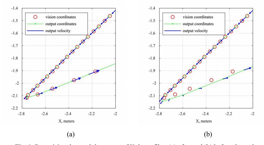
• 1.Kalman filter for ball tracking was identical to the one, used for robot tracking, therefore invalid filter behavior took place when the ball bounced from a robot (friendly or enemy): in the output, ball velocity change was smooth and ball trajectory was a smooth curve as well, while in reality velocity changed in a jump manner and, accordingly, the trajectory contained a sharp corner. In such case, the difference between the actual and output coordinates of the ball could significantly exceed the error of the vision system.
• 2.In Kalman filter [1] for friendly robots, there was no consideration of robot control vector $u_k$, which should depend on the set translational and angular velocities. Instead, an input-free state-transition equation $x_k=F^k x^{k-1}+w^k$ was assumed in the model. Translational and angular acceleration, emanating from control inputs, were counted for as mutually independent "noisy" increments of velocity, by specifying appropriate diagonal entries of the covariance matrix $Q^k$ of process noise vector $w^k$. Such approach leads to a limited precision of both position and velocity measurements: the entries of $Q^k$ should be assigned in compliance with maximal admitted translational and angular accelerations of the robot (otherwise filter output will feature considerable delays in case of intensive maneuvers), therefore a jitter in vision data is inevitably transformed into oscillations of the components of $x^k$.
• 3.Ball interception algorithm did not include the prediction of ball kinematics; therefore, the intercepting robot was always directed to the current ball location – such tactics is nonoptimal and leads to the loss of time, especially when the ball is moving towards the robot.
• 4.Instability of high-speed robot motion perpendicular to its symmetry axis namely, the presence of angular and translational oscillations – resulted in interception failure when the ball to be intercepted was moving (nearly) perpendicular to kicking direction. The intercepting robot tended to push the ball by its cover rather than properly align its kicker with the ball and shoot.

While the problem outlined in item 2 of the list is under intensive study at the time, significant improvements have been made to remove or alleviate the shortcomings mentioned in items 1, 3 and 4. Subsections below describe the relevant algorithmic updates.

2.1. Ball Kalman Filter

It is desirable that the ball tracking algorithm satisfies two qualitative requirements:

• to maintain high precision of position and velocity measurement when the ball is in free motion, i.e. rolls across the field without being touched;
• to avoid "transient processes" in output data, as outlined in item 1 of the drawbacks list above, when the ball bounces from a robot.

Satisfying both requirements, using the basic implementation of Kalman filter with constant state-transition parameters (transition matrix $F_k$ and noise covariance matrix $Q_k$) is troublesome, but the dilemma is easily resolvable by assigning $Q_k$ entries at each step according to mutual location of the ball and all robots in the field. The key idea is to consider ball velocity dynamics as practically undetermined if the ball gets too close to any robot. State-transition equation retains simple form

$$X_{k} = F_{k} X_{k-1} + W_{k} \quad , \tag{1}$$

where $$x = \begin{pmatrix} X \ Y \ V_x \ V_y \end{pmatrix}$$ , $F = \begin{pmatrix} 1 & 0 & \Delta t & 0 \ 0 & 1 & 0 & \Delta t \ 0 & 0 & 1 & 0 \ 0 & 0 & 0 & 1 \end{pmatrix}$ , (2)

with $\Delta t$ standing for the interval between the current and previous data bursts from vision system: $\Delta t = t_k - t_{k-1}$. Formulas (1) and (2) result from the continuous model of motion

$$\dot{r}(t) = V(t)$$ , $\dot{V}(t) = a(t)$ ,

where a is the (de)acceleration due to friction or contact with a robot, as its discrete analogue under the simplifying assumption that the components of a are independent zero-mean Gaussian random variables. Covariance matrix of process noises $W_k$ is determined as

$$Q_k = \begin{pmatrix} 0 & 0 & 0 & 0 \ 0 & 0 & 0 & 0 \ 0 & 0 & \sigma_k^{\square} & 0 \ 0 & 0 & 0 & \sigma_k^{\square} \end{pmatrix}$$

where $$\sigma_{k}^{\square} = \begin{cases} a_{\text{fric}} \Delta t / 10, & \Delta R_{\text{min}} < r_{\text{r.b.}} + \varepsilon, \ V_{\text{b.max}}, & \Delta R_{\text{min}} \ge r_{\text{r.b.}} + \varepsilon, \end{cases}$$ (3)

$a_{\rm fric}$ is the ball typical deceleration (about 1 m/s²) due to rolling friction, $V_{\rm b.max}$ — maximal admitted shooting speed (8 m/s), $r_{\rm r.b.}$ — the sum of robot and ball radii (11 cm), $\varepsilon$ — some tolerance, around 1 cm, and

$\Delta R_{\min} = \min \left[ \Delta R_{\text{vis}}, \Delta R_{\text{pred}} \right]$ is the minimum between the distance $\Delta R_{\text{vis}}$ to the closest robot according to the latest raw vision data and the minimal predicted distance $\Delta R_{\text{pred}}$. The latter is computed for each robot as

$$\Delta R_{\text{pred}} = \left| r_{k-1}^{\text{b}} - r_{k-1}^{\text{r}} + (V_{k-1}^{\text{b}} - V_{k-1}^{\text{r}}) \Delta t \right|$$

with $r_{\square}^{\rm b}$ and $r_{\square}^{\rm r}$ respectively denoting the ball and robot coordinates, and $V_{\square}^{\rm b}$ and $V_{\square}^{\rm r}$ — their velocities, all taken from the previous Kalman filter output. Symbol "≈" in formula (3) is used, as the exact values of the parameters should be selected experimentally. Note that before contact with a robot was taken into account, the upper option in formula (3), with an increased value of $a_{\rm fric}$, had been used unconditionally.

The preference of the outlined algorithm is illustrated in Fig. 1, which depicts the trajectory of the ball kicked by a robot (at the bottom-left corner). Fig. 1a and Fig. 1b present tracking results with and without the update respectively. It is clear that tracking performance at the stage following the kick has significantly improved.

2.1. Rolling Friction Analysis and Prediction of Ball Coordinates

An accurate robot guidance to a point, where the free-rolling ball will be located after a certain period of time, requires knowledge about the law of ball motion. The dominant force affecting the ball results from rolling friction. Theoretically, such force should always be directed opposite to ball forward motion and have constant magnitude. Respectively, ball deceleration should be constant while the ball is rolling. However, as confirmed by experiments, the field carpet causes deceleration strongly dependent on ball speed: it ranges from around 0.3 m/s² for a slow-moving ball, and up to 10 m/s² at high speeds. Therefore, the assumption of constant deceleration cannot be used for efficient prediction.

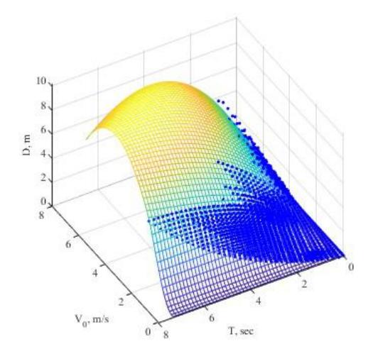
In order to facilitate prediction, we designed a special estimation method for function $D(T, V^0)$, where $D$, $T$ and $V^0$ stands for the distance to be travelled by the ball with current (initial) speed $V^0$ within $T$ seconds. The method was based on two-dimensional (2-D) polynomial fitting [2]. In the experiments, the ball was launched across the field many times, with different initial speeds and in different directions. The recorded vision data (ball coordinates) were processed in MATLAB: travelled distance at each free-motion fragment was approximated by the 5th degree polynomial (the order was chosen heuristically), which enabled the computation of jitter-free speed. The interpolated data arrays $\Delta r_j=\Delta r(t^j)$ and $V^j=V(t^j)$, where $\Delta r$ is the distance from the starting point of the fragment and $j=1,2,…, J$, we converted into samples {$T, V^0, D$}$^n$ with $j=1,2,…, N$. Since any pair of index values $j$ could be used to create the sample, a total of $N=J(J−1)/2$ samples were generated from a single free-motion fragment. The data from all fragments was collected into a joint array, and the function $D(T, V^0)$ was estimated as a 5th degree (again, the order was chosen heuristically) 2-D polynomial

$$D(T,V_0) = \sum_{m+k \le 5} c_{mk} T^m V_0^k$$

using the least squares principle. Estimation results are depicted in Fig. 2, where the smooth mesh surface is the graph of the 2-D polynomial, and the blue dots indicate the samples {$T, V^0, D$}, which are scattered below the surface as well as above it. It should be noted that the area, where both $T$ and $V^0$ are large, is of no practical importance, therefore the behavior of the polynomial in such area can be ignored.

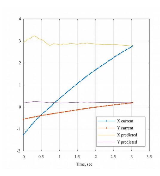
On the basis of $D(T, V^0)$, the prediction algorithm was developed. The effectiveness of this algorithm is illustrated by Fig. 3, where the predicted ball coordinates for the initial prediction time of 3 seconds (a relatively large value was selected exclusively to demonstrate the stability of prediction within a wide range of time intervals) are plotted along with its actual coordinates.

2.2. Ball Interception Algorithm

As mentioned in the beginning of the section, the alignment of robot velocity with that of the ball in order to guarantee a smooth approach of the interceptor to the ball resulted in the failure of interception in certain cases, owing to an unstable robot motion when the set velocity was perpendicular to the symmetry axis of the robot. The problem has been solved by the replacement of such method with robot guidance to a predicted point via a path, where side motion (with respect to the axis of symmetry) is avoided at the final stage of interception. This technique was enabled by the improvement in ball prediction (see subsection 2.1).

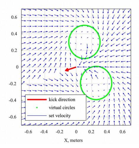
The new algorithm, guiding an intercepting robot to the ball, exploits geometric approach in order to make the robot move along the desired path. Two symmetrically located virtual circles 20 cm in radius are introduced behind the interception point with respect to the kick direction, and the set velocity is assigned in such a way that the robot should move around one of these circles unless it is already in the narrow (30°) angular sector between the circles. For the sake of brevity, instead of presenting tedious multi-case formulas of the algorithm, we provide its graphical description by Fig. 4, presenting the field of set velocity on the grid of robot locations around the interception point. It is taken into account that, on the one hand, the robot should move with its maximal speed where possible and that, on the other hand, robot motion along a circle of the indicated radius is possible only at a moderate speed (about 0.5 m/s), therefore the algorithm guides the robot to decelerate smoothly when approaching to the circle and accelerate after the sector between the circles is reached. Also, the set robot speed is adjusted in compliance with the time left to the occurrence of the ball in the interception point, so that the robot intersects with the ball exactly on time.

3. Electronic Design

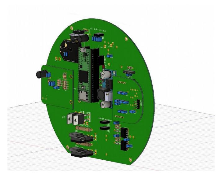
This year, previous circuit version has been improved. The main objective of the changes focused on efficiency and reliability. Errors in the previous circuit were eliminated and these changes increased efficiency. Moreover, new daughter boards were added to the circuit. 3D model of the circuit has designed in AUTODESK EAGLE and pushed into Fusion 360 to give design planning.

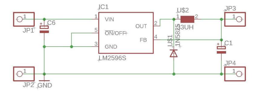
The standard 7805 regulator is removed from the main circuit. Main reason for removing the regulator is that it was causing problems to supply Teensy. LM2596 step down voltage regulator was used instead of the standard 7805 regulator. The new stepdown regulator which is used in the main circuit can provide 3A-5V output. The old voltage regulator 7805's max output current was 1A, which results an advantage for the new power board [3]. With this change, the problems in teensy were solved and efficiency increased. Because the teensy is more efficient and reliable with a stable voltage. So, the regulator that used provides this stability. Moreover, the layout of the main circuit has a total make over to increase reliability. The high voltage path has been decreased. Furthermore, the communication shield XBEE's location has changed. Old location was nearby the high voltage path and solenoid sockets. Since it was near the high voltage path, XBEE was affected by the magnetic field thus causing some communication problems.

Topology of the charger circuit remains same with last years. However, issues have been fixed in the previous circuit by changing the PCB layout. While changing the PCB layout, the aim was to increase reliability and safety. LT3750 capacitor charger controller is a sensitive device which needed to be designed the PCB layout carefully. To increase the layout of the MOSFET's drain cause leakage inductance of transformer. Furthermore, regular capacitors are changed to special capacitors which have low ESR. Another improvement is the changing of input voltage of digital isolator ADUM 7441. Teensy digital pins have a 3.3 V tolerate. More than 3.3 V can destroy the teensy. So, input supply voltage of the ADUM 7441 which is isolator between teensy and DACs has decreased to 3.3 V from 5 V.

4. Mechanical Design

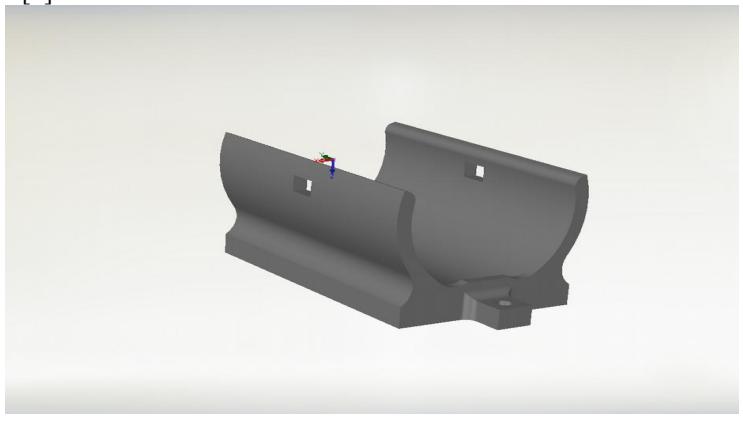
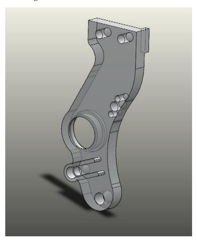
This year there are a few changes in the mechanical designs of robots. These new changes helped robots to improve stability and strength. Structure of robots was reinforced with new designs of 3D printed parts and become more mechanically robust. Dribbler and kicker mechanisms are renewed this year, also robots now have a capacitor holder [4].

Old generation robots had stability problems due to capacitor was not properly mounted on the structure of the robot and robot collisions during the games effects the center of gravity making robots unstable and even sometimes falling. However, this year with the help of a newly designed capacitor holder robots are going to achieve this problem and become much more stable during the games.

4.1. Dribbler and Kicker Mechanism Improvements

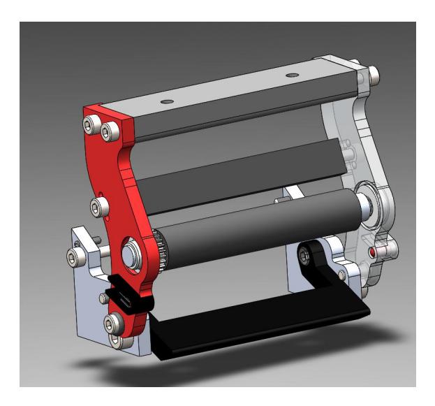
This year, robots have upgraded dribbler and kicker mechanisms. Their design has been developed and reinforced with newly designed arms and beam support parts. New design of dribbler is more inside of the robot thus eliminates rare occurrence of losing ball from the vision. Also, sometimes kicker was not doing kicks properly due to misplacement of the solenoid, now that problem was fixed as well.

4.2. New Arms Design

Robots LEDs are constantly broken because of the robot collisions. After doing excessive collision tests it is noticed that newly designed arms cut off this break problem.

5. Software

In the software the team is using the same mechanics before which is Behaviour Trees. Each tree is assigned a goal, that will be achieved. The robot behavior is a control law that satisfies a set of constraints to achieve a particular goal. Each behavior is defined by the set of actions. BTs perform a number of artificial intelligence (AI) techniques such as Finite State Machines, Scheduling, Planning, and Action Execution[5][6].

References

1. Simon, D.: Optimal State Estimation: Kalman, H Infinity, and Nonlinear Approaches. Wiley-Interscience (2006)
2. Mathews, J.H., Fink, K.K.: Numerical Mathods Using Matlab. 4th edn. Pearson, New Jersey (2004)
3. R.H. Abiyev, N. Akkaya, M. Arici, A. Cagman, S. Huseyin, C. Musaogullari, A. Turk, G. Say, T. Yirtici, B. Yilmaz, E. Aytac: Team Description Paper 2018, Robocup SSL, Montreal, Canada (2018).
4. R.H. Abiyev, I. Gunsel, N. Akkaya, M. Arici, A. Cagman, S. Huseyin, B. Yilmaz, E. Aytac: Team Description Paper 2017, Robocup SSL, Nagoya, Japan (2017).
5. R.H.Abiyev, I.Günsel, N.Akkaya, E.Aytac, A.Çağman and S.Abizada, "Robot Soccer Control Using Behaviour Trees and Fuzzy Logic", in Proc. 12th Int. Conf. on Application of Fuzzy Systems and Soft Computing, ICAFS 2016, Book Series: Procedia Computer Science, vol.102, pp. 477-484, 2016.
6. Rahib H.Abiyev, Nurullah Akkaya, Ersin Aytac, Dogan Ibrahim. Behaviour Tree Based Control For Efficient Navigation of Holonomic Robots. International Journal of Robotics and Automation, Volume: 29 Issue: 1, 2014, pp: 44-57.