RoboJackets 2019 Team Description Paper

J. Almagro, C. Avidano, C. Lindbeck, J. Neiger, Z. Olkin, E. Peterson, K. Stachowicz, W. Stuckey, M. White, M. Woodward, G. P. Burdell

Georgia Institute of Technology

Abstract The RoboJackets RoboCup SSL team was founded in 2007 and has competed every year since. The team's objective this year was to improve the mechanical and electrical robustness of the overall system based on lessons learned from competition and continuous testing. In parallel, the team added more planning capabilities to the team's software and added firmware features. This paper describes these fleet upgrades and the progress made on their implementation.

1 Mechanical

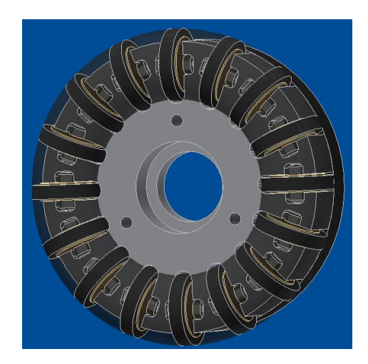
For this iteration of the wheel the focus was on nailing down the tolerance for the rollers as well as the bearing. In previous years there were issues with the efficiency of the wheels which led to problems with motion control of the robots. To combat the lack of adequate tolerancing, manufacturing was outsourced and the design was modified to ensure that even if the tolerance is too large the bearing will stay in place. The modification took place in the form of a pocket as seen in Figure 1. This pocket is then filled with the bearing and sandwiched with the top plate of the wheel. This allowed for smaller tolerance estimates.

1.1 Wheel

For this iteration of the wheel the focus was on nailing down the tolerance for the rollers as well as the bearing. In previous years there were issues with the efficiency of the wheels which led to problems with motion control of the robots. To combat the lack of adequate tolerancing, manufacturing was outsourced and the design was modified to ensure that even if the tolerance is too large the bearing will stay in place. The modification took place in the form of a pocket as seen in Figure 1. This pocket is then filled with the bearing and sandwiched with the top plate of the wheel. This allowed for smaller tolerance estimates.

1.2 Chipper

This year a chipper was created to be able to properly restart on direct and indirect kicks. Due to the previous designs for the other sub-assemblies the traditional square solenoid would not fit into the robot effectively, other designs were investigated. Inspiration for the final design was drawn from the RoboJackets 2011 fleet design. This led to a design with the chipper solenoid mounted on top of the kicker solenoid.

Boot

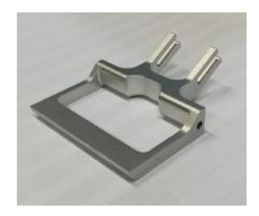
To ensure that the boot would not cause interference with the kicker two different configurations were considered. The first design was to manufacture the boot in such a way that it was always behind the kicker. This was not used due to the previously designed kicker boot being too large to contort the chipper boot around without making it too weak. In essence, the chipper boot would have had to go under the kicker head to not interfere, which would have led to a thickness of the boot that would not be robust enough to withstand repeated impacts with the ball. Overall, the design would be over complicated for minimal return on investment. This led to the second design which was to place a hole in the chipper boot to ensure that the kicker would not interfere with the chipper.

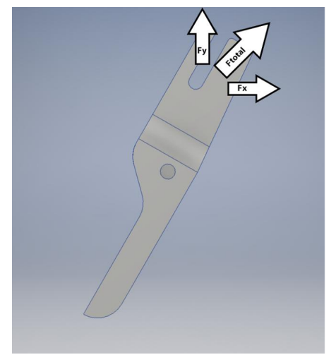
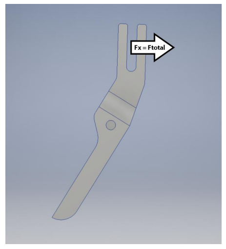
Once it was decided to use the hole based design, work began on optimizing the angle of the connection point between the boot and the chipper rod. According to the principles of dynamics the closer the angle of interaction is to 90 degrees, the smoother the force transfer.

Using this idea four different chipper boots were designed to test the theory empirically. The last iteration on the design worked acceptably, however a final design was created to make sure that it could not be further optimized. This design changed the angle to a full 90 degrees and lowered the point of rotation to increase the moment arm. However, when this design was tested under the same conditions it was found to under-perform. The hypothesis for why it underperformed is due to the smaller mass of the boot necessitated by the new design. The decrease in mass led to a lesser momentum transfer as defined in Equation 1.

$$v_2 = (2 * m_1 * v_1) / (m_1 + m_2) \tag{1}$$

Manufacturing for this component was once again outsourced for tighter tolerances and a nicer finish.

Plunger

The plunger for the chipper is fairly straightforward. For the back part, which is made of aluminum, the same design from the kicker was used. For the front of the plunger which interacts with the boot of the chipper a cross bar was added that fits into the boot to ensure that it can be pulled back, and thus chip the ball. To achieve this a rod was welded into a groove in the steel plunger.

1.3 Dribbler

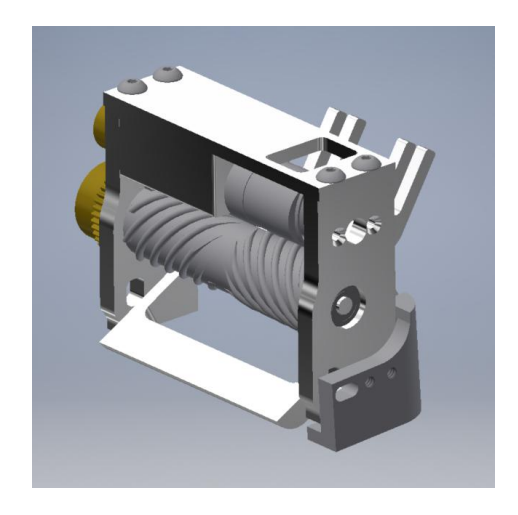
Last year the dribbler design did not work very well for receiving passes. This led to the development a dribbler that could dampen the impact of the ball so catching is effective. Inspiration was taken from ZJUs 2018 dampening dribbler design [1]. This meant that the pivot point was placed at the base of the robot in conjunction with the same part that held the chipper. The damping element was attached at the top of the dribbler in contact with the midplate.

1.4 Rubber Roller

Another issue with the robot that was noticed during competition was that the roller did not actually grip the ball to maintain control while dribbling. Originally a foam was used since some short testing revealed that it gripped the ball very well and had a moderate damping effect. However, the material was not durable enough which caused it to disintegrate when pressed too hard against the ball while dribbling. After some testing, Urethane with a Shore Hardness of 30 was chosen as it is a material better suited to handling the stresses that the rubber roller experiences. After extensive stress testing it was determined that the material was adequate and would hold up.

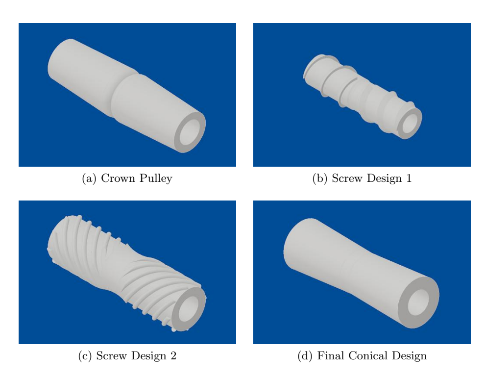
The other aspect that needed testing was the centering capabilities of the roller. For this a couple of different designs were tested. The first was a crown pulley style roller which ended up pushing the ball to the sides of the dribbler rather than the center. Two different screw designs were also tested that worked decently well, however due to the delicate geometries they would break down over time and eventually lose their ability to center the ball. The final design that was tested was a standard conical design to smoothly transfer the ball to the center of the dribbler. This is the design was found to be the most consistent over time.

2 Electrical

The control and kicker electrical boards this year are based off the design from 2018 with improvements to make the system more robust and to collect more data. The new microcontroller board is based off of the Mbed microcontroller that was previously used.

2.1 Microcontroller Board

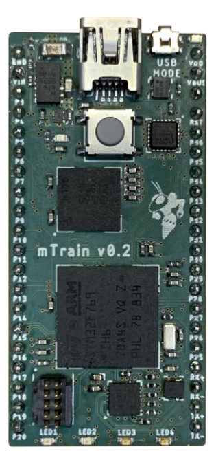
As more onboard motion control was added to the robots the limits of the current microcontroller were reached. An existing suitable replacement board was not found, so a new microcontroller board was created to replace the previous Mbed board. The major change for this new board was upgrading the microcontroller chip from an ARM Cortex-M3 to an ARM-Cortex M7. This will allow for lower latency and higher throughput motion control processing. The enabling features are integer vector support, a hardware floating-point unit, and hardware floating point vector support. There are a number of other advantages to the new Cortex-M7 chip such as faster IO interfaces to communicate with on board chips.

On the new board, a high-speed USB interface chip was added for Hi-Speed USB 2.0 communication to be used for debugging and radio communication. A 256 MB flash chip was added to store files such as binaries to program other components on the robot. A 256 Mb RAM chip was added for future use with more complex motion control. The JTAG port was also exposed which will allow for more precise debugging compared to the past Mbed board.

In order to easily write code for the new microcontroller, an API was written similar to the one that was provided with the Mbed. One of the main advantages of the Mbed was being able to easily write code and program the board. To have a similar convenience on the new board a bootloader was written to easily program the board over Hi-Speed USB.

2.2 Control Board

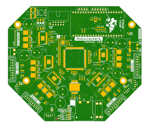
The control board has been primarily modified to better support the new motion control system for the robots. Support for the Mbed microcontroller has been switched to the new microcontroller which has the hardware units necessary for increased computational speed. Additionally, current-sense resistors were added in-line to the motors that lead to ADCs which will be read by the FPGA to provide data for the motion control system. The current sense-resistors are each connected to a current-sense amplifier, the TI INA240, which enables PWM rejection with a high common mode rejection ratio in order to get accurate voltage drops across the shunt resistors.

All of the large components including the battery connector and bulk capacitors for the motors have been moved to the top of the board to increase space efficiency and make room for a chipper. The bulk capacitors were changed to through-hole capacitors because the surface mounted capacitors would often get ripped off of the board. A connector has been added to the board to support serial communication for future off-robot ball detection. Another connector and motor driver was added to support a motor that would rotate the kicker assembly. Lastly, the radio connector is going to be switched to a radio agnostic connector so there are multiple options for what type of radio is used based off of performance and reliability.

2.3 Kicker Board

This kicker board iteration is mostly designed to address issues of reliability from the previous version. It also places a greater emphasis on independent operation from the control board, which makes debugging easier and allows for operation by mechanical engineers that dont want to boot the entire software stack to test.

The new board will be switching to the LT3751 from the LT3757 as the primary switch mode regulator. The primary benefit is a capacitor charging mode that uses current measurements from the primary side as feedback. This eliminates a feedback line from the high voltage side, removing a point of failure where high voltage can damage low voltage systems. It also features over and under voltage lockouts for added safety. Performance is also improved. The primary side current is increased to 50A from 20A and total capacitance is increased to 4000uF from 3440uF. This significantly reduces charge time and increases the frequency and power with which the robot can kick.

The microcontroller is upgraded to an ATmega32A from an ATtiny167. Board features demanded the additional IO capabilities, but compute performance is similar. We use this line of microcontroller because it is easy to flash firmware over the same SPI lines that are used for communication between kicker and control boards. This is something mostly absent from the ARM line of embedded controllers. Additional measures are taken to protect the onboard microcontroller: TVS diodes have been added to all power rails and RC snubbers with an aggressive cutoff frequency to mitigate ringing on the LT3751 control lines. This ringing was observed on the previous kicker board version and may have been a source of damage.

Power FETs used for solenoid discharge are replaced with IGBTs. While IGBTs have a slower switching frequency, they support much higher currents. The additional supported current adds a wide margin for better reliability and also allows testing of solenoids with lower impedance. FET gates are now driven by a dedicated regulated power rail which helps protect IGBT gates from any potential unmitigated spikes on the primary battery power rail.

2.4 Radio

The commercially available ISM-43340 dual band Wi-Fi radio is being evaluated for usage in future competitions. Previous communication with the robot used Decawave radios via the DWM1000 module. This proved to be unreliable as Decawaves rely on multi-path propagation to reconstruct packs in high noise and non-Line-of-Sight (LOS) transmission. The wide open venues do not propagate as many paths compared to hallways and smaller rooms, resulting in significantly decreased reliability when LOS is broken. Wifi is a ubiquitous technology and historically the 2.4 GHz spectrum is highly contested in public spaces. The ISM-43340 is begin evaluated with an emphasis on a business class access point and router to more properly address issues with a contested spectrum. The robots will use two modules per platform. Many Division A teams use redundant radios to help alleviate LOS and stochastic environmental issues when at competition. Initial testing is reporting 0.6ms average round-trip latency on TCP transmissions in a contested 5GHz transmission.

3 Software

3.1 Robot / Ball Filter

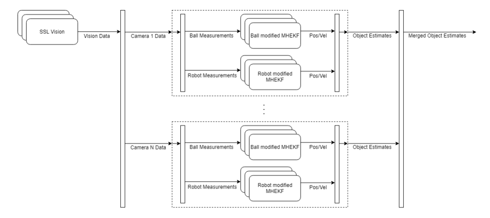
The robot / ball filter converts the camera measurements from SSL vision [2] and produces a singular best estimate of the positions / velocities of the objects themselves. This is done through a camera centric modified Multi-Hypothesis Extended Kalman Filter (MHEKF) [3].

Modified MHEKF

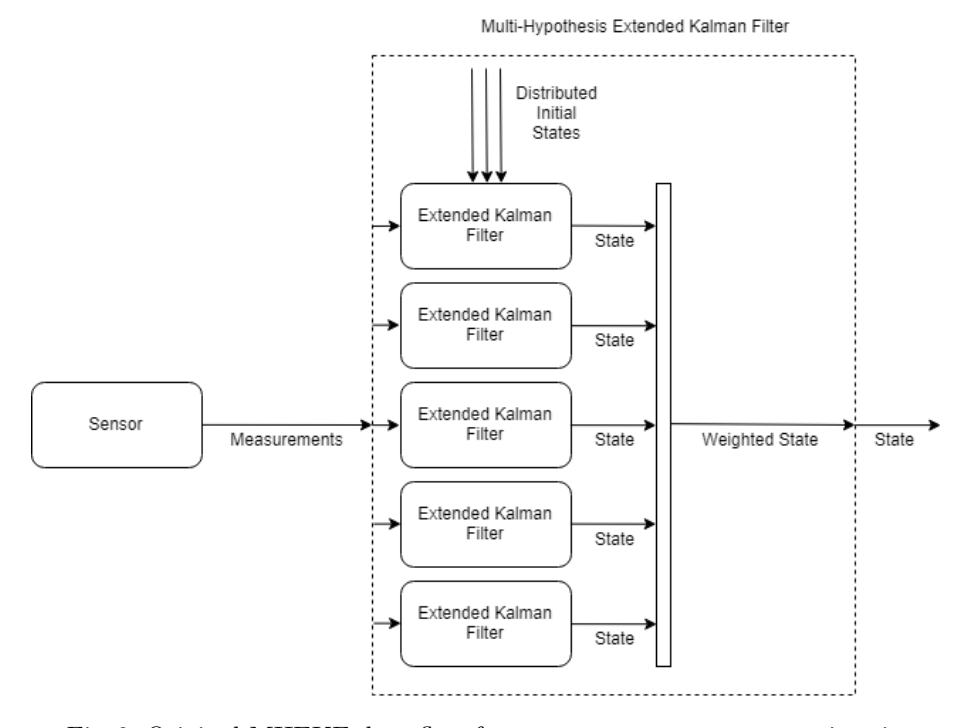
A significant challenge for the robot / ball filter is intelligently dealing with multiple measurements in a single frame which may include many false positives. Additionally, the false positives measured across multiple frames are not statistically independent allowing for multiple perceived trajectories for objects. The original MHEKF [3] feeds a single measurement through a range of evenly distributed extended Kalman filters (EKF). This ensures at least one of the EKFs properly converges to the true state.

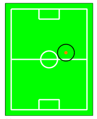
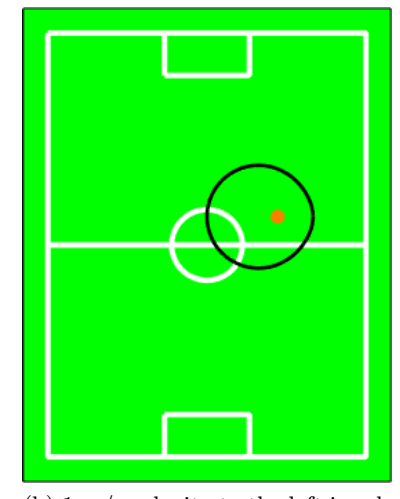
Since a simple linear integrator model was chosen as the base for each of the objects plant models, a single Kalman Filter (KF) in the modified MHEKF set is initialized at each of the measurements in a single frame. If there is already a single KF in the modified MHEKF set in the vicinity of the measurement, the measurement is then used as the observation for that specific KF in the set. The overall data flow from SSL Vision through the estimates can be seen in Figure 9. In a general system where the model matches the process the covariance can be used to reject unlikely measurements. Due to large accelerations of both the balls and robots a static distance cutoff and a velocity scale factor are used as seen in Figure 10.

In the case of multiple measurements being applied to a single KF, the measurements are simply averaged. Additionally, to improve movement across cameras, the initial velocities of the KFs are set to the previous best estimate of the velocity of the object. This allows smooth estimation transitions between cameras.

Merging Across Cameras

The modified MHEKF produces a set of estimates for each trajectory that has been detected for every object. At the global level, the most updated KF is taken from each camera. This set is then combined based on a simple weighted average. The frequency of update as well as the covariance of the filter influence the importance of the states in the average as seen in equation 2. $x^i$ is the position, velocity, orientation, and angular velocity of the KFs in the most updated set. $\sigma^i$ is the covariance of the position, velocity, orientation, and angular velocity state in the KFs. $u^i$ is a scale factor representing how updated this KF is. The larger the scale factor, the more it has been updated, with a minimum value of 1. N is the number of KFs in the most updated set. $\alpha$ is a configuration coefficient that is set between one and two to properly weight the average. $x^w$ is the resulting state using the best estimate of the object overall.

$$x_w = \sum_{i=1}^{N} \left(\frac{1}{u_i}\sigma_i\right)^{-\alpha} x_i \tag{2}$$

Results

The modified MHEKF ball/robot filter is a significant improvement over the simple complementary filter used initially. The improved filter reacts within eight frames compared to the 12 frames with the complementary filter. Additionally, the resulting velocity profile tracks the expected profile significantly better. The transition between the back-spin phase and the rolling phase of the ball during a kick is clearly seen in the improved filter.

3.2 Motion Planning with Acceleration Constraints

The acceleration limitations of the robots are primarily due to wheel slippage. Accounting for this limitation in the path planning layer after the obstacle avoidance allows for a more consistent motion as well as less reliance on both the hard acceleration limits on the robot and the motion control on a positional level. Two methods are explored to account for this limitation. The first breaks a smooth path generated by the existing obstacle-avoidance step into many intervals and limits wheel acceleration to feasible values along each interval while maximizing tangential acceleration along the path. The second method exploits the linearity of the acceleration limitations in the wheel frames to produce a set of linear constraints allowing for a cubic polynomial trajectory fit to produce a path given a sparse set of waypoints from the path planning layer.

Three-Pass Method

In the three-pass method for matching wheel acceleration constraints, an existing path planned previously through a rapidly-exploring random tree or another similar method is re-parametrized so that the robot follows the path without exceeding wheel acceleration constraints.

Let a path be a function: $\gamma:[0,1]\to\mathbb{R}^3$ such that $\gamma(s)=(x(s),y(s),\theta(s))$. The goal is to create a function $\sigma:\mathbb{R}\to[0,1]$ such that $\gamma(\sigma(t))$ is a path that the robot can actually follow, with acceleration constraints given by the wheel constraints on the robot.

In the three-pass method this function is determined numerically: a table look-up (in which [0,1] is partitioned into many segments of length ds) is created and filled in via a forwards and backwards pass to find actual values for $\sigma(t)$. The path is first broken up into a series of small segments, each of which is approximated as an arc with constant curvature, over which the accelerations on each of the wheels are held constant.

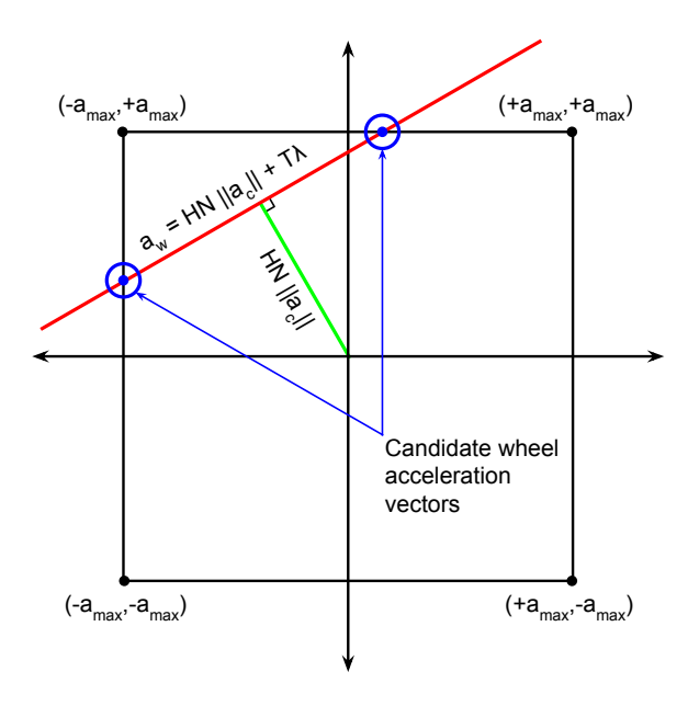
The main active constraint is a box constraint on the wheels accelerations. This creates a feasible region $U = [-a_{max}, a_{max}]^4 \subset \mathbb{R}^4$ from which the wheel accelerations may be chosen. In addition, for a given segment, there is the constraint of constant curvature $\kappa$. Assuming the segment has roughly constant velocity v, the magnitude of the centripetal acceleration can be written as $||a_c|| = \kappa v^2$. Then, the goal is to find the tangential acceleration $a_t = \lambda T$ where $\lambda \in \mathbb{R}$ is the magnitude of the tangential acceleration and $T \in \mathbb{R}^3$ is the vector (with x, y, and $\theta$ components, where the x and y components together have unit magnitude) tangent to $\gamma$ at a given segment. These values create another constraint on acceleration: a line written as $a_{body} = \kappa v^2 N + \lambda T$ (where N is the unit normal to the curve with a zero $\theta$ component) that describes the set of all accelerations that will still result in the robot following the path. Let $H \in \mathbb{R}^{4 \times 3}$ be the linear transformation from robot-space differentials $(dx, dy, \text{ and } d\theta)$ to wheel-space differentials $(dw_i)$, assuming $\phi_i$ as the robot-centric angle of the ith wheel and R is the robot's radius (measured from the center of turning to the wheels):

$$\begin{bmatrix} dw_1 \ dw_2 \ dw_3 \ dw_4 \end{bmatrix} = H \begin{bmatrix} dx \ dy \ d\theta \end{bmatrix}$$ (3)

$$H = \begin{bmatrix} \sin \phi_1 \cos \phi_1 & R \ \sin \phi_2 \cos \phi_2 & R \ \sin \phi_3 \cos \phi_3 & R \ \sin \phi_4 \cos \phi_4 & R \end{bmatrix}$$ (4)

Because $a_{wheel} = Ha_{body}$ for as the transformation between robot-space differentials and wheel-space differentials, this line can be transformed into wheel space. Figure 11 shows the reduced two-wheel problem for visualization's sake, where acceleration is chosen from $\mathbb{R}^2$ instead of $\mathbb{R}^4$.

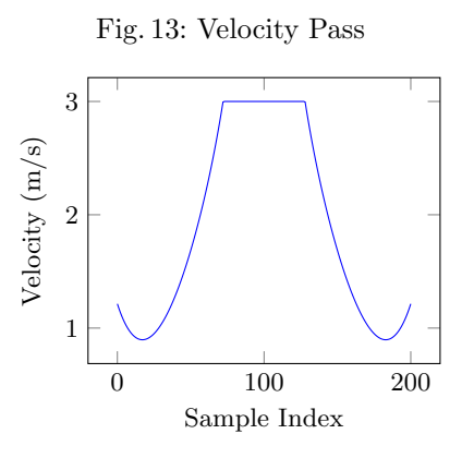
In the velocity pass, an upper bound on the forward velocity at each segment on the path is found by assuming zero tangential acceleration and maximizing the magnitude of $||a_c||$ while keeping wheel accelerations in the feasible region. In addition, this pass provides the option to limit the robots maximum velocity to a fixed maximum, in the case of zero curvature.

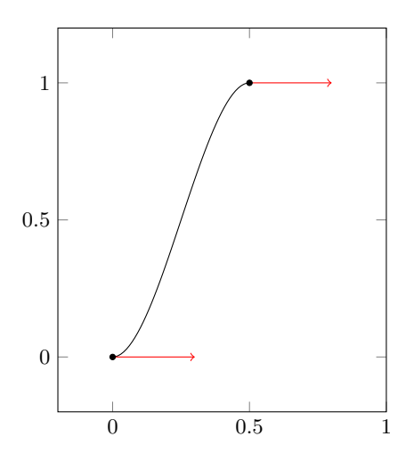
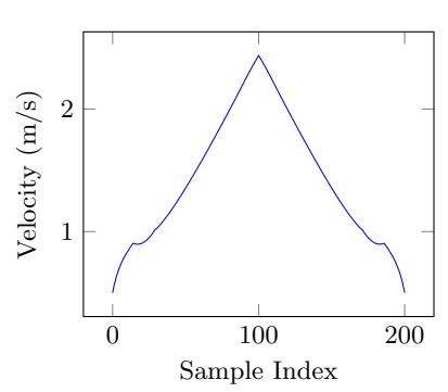
Figure 13 shows the resulting velocities after the velocity pass plotted against the sample index (the index of the segment ds) when the method is applied to a s-curve starting at the origin with velocity (0.5,0,0) and ending at (0.5,1,0) with velocity (0.5,0,0), as shown in 12.

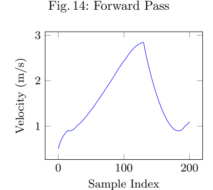
Next, the forward pass is carried out. Examining figure 11, the intersection with largest (most positive) $\lambda$, which signifies forward acceleration along the path, is chosen (assuming T is chosen to point in the direction of motion). This gives the tangential acceleration along the path, which can be used to calculate the speed at the end of this segment as well as the time taken to follow the segment. This process is carried out iteratively along the path, with each segment using the previous states final velocity as its initial velocity. Figure 14 shows the result of the forward pass.

However, this velocity profile does not respect acceleration constraints while decelerating — note the sharp decrease in velocity once the forward pass is only limited by the centripetal acceleration required to maintain velocity going along a sharp curve. To fix this, the forwards pass is run in reverse, as shown in Figure 15.

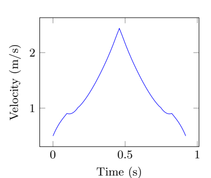
This gives an estimated velocity at the boundary of each segment of the interval [0, 1]. Then, the dt for each segment can be found by dividing arc length by average velocity, and this variable can be integrated to find the function $t = \sigma^{-1}(s)$, which can be easily interpolated to find $\sigma(t)$. Plotted against the time axis, the final velocity profile is shown in figure 16.

QP Formulation

A QP (quadratic programming) method of generating trajectories between a sparse set of waypoints was also explored. In this method, a receding horizon planner is used to fit the coefficients of a cubic parametric polynomial in time in order to minimize the terminal sum-of-squares error while maintaining wheel acceleration constraints at the beginning and end of the profile.

In a cubic polynomial, the second derivative (acceleration) is a first-order polynomial in time. It is smooth and has a non-vanishing derivative, so the extrema exist at the boundaries. Therefore, for any coefficients, acceleration will be highest at the beginning and end - so it is only necessary to constrain acceleration at those points.

The goal is to fit three equations:

$$x(t) = c_{0x} + c_{1x}t + c_{2x}t^2 + c_{3x}t^3$$ (5)

$$y(t) = c_{0u} + c_{1u}t + c_{2u}t^2 + c_{3u}t^3$$ (6)

$$\theta(t) = c_{0\theta} + c_{1\theta}t + c_{2\theta}t^2 + c_{3\theta}t^3 \tag{7}$$

Because the robots initial position and velocity (and by proxy $c_{0*}$ and $c_{1*}$) are fixed, it is only necessary to solve for $c_{2*}, c_{3*}$. The final positions and velocities are as follows (equations for y and $\theta$ are analogous):

$$x(T) - (x(0) + x'(0)T) = c_{2x}T^2 + c_{3x}T^3$$ (8)

$$x'(T) - x'(0) = 2c_{2x}T + 3c_{3x}T^2$$ (9)

These linear dependencies can be expressed in matrix form as $\overrightarrow{x} - \overrightarrow{x'}0 = P \overrightarrow{c}$, where $\overrightarrow{x}$ is the vector of final positions, $\overrightarrow{x}$ represents the effects of $c{0*}, c_{1*}$ on the final state and velocities and $\overrightarrow{c}$ is the vector of $c_{2*}, c_{3*}$:

$$\overrightarrow{x} = \begin{bmatrix} x(T) \ x'(T) \ y(T) \ y(T) \ \theta(T) \ \theta'(T) \end{bmatrix}, \overrightarrow{x}_0 = \begin{bmatrix} x(0) + x'(0)T \ x'(0) \ y(0) + y'(0)T \ y'(0) \ \theta(0) + \theta'(0)T \end{bmatrix}, P = \begin{bmatrix} T^2 & T^3 & 0 & 0 & 0 & 0 \ 2T & 3T^2 & 0 & 0 & 0 & 0 \ 0 & 0 & T^2 & T^3 & 0 & 0 \ 0 & 0 & 2T & 3T^2 & 0 & 0 \ 0 & 0 & 0 & 0 & T^2 & T^3 \ 0 & 0 & 0 & 0 & 2T & 3T^2 \end{bmatrix}$$

$$\overrightarrow{x} - \overrightarrow{x}_0 = P \overrightarrow{c} \tag{10}$$

In addition (as in the multi-pass constraints method described above) there is a matrix H transforming from body-space differentials to wheel-space and a maximum wheel acceleration $\overrightarrow{a}_{max}$. Differentiating Equation 7 results in the following transformation (also expressible in matrix form - call this matrix A) from coefficients to initial and final acceleration:

$$x''(0) = 2c_{2x}$$ (11)

$$x''(T) = 2c_{2x} + 6c_{3x}T$$ (12)

$$A = \begin{bmatrix} 2 & 0 & 0 & 0 & 0 & 0 \ 2 & 6T & 0 & 0 & 0 & 0 \ 0 & 0 & 2 & 0 & 0 & 0 \ 0 & 0 & 2 & 6T & 0 & 0 \ 0 & 0 & 0 & 0 & 2 & 0 \ 0 & 0 & 0 & 0 & 2 & 6T \end{bmatrix}$$ (13)

Let $\overrightarrow{g}$ be the desired final state and $Q \in \mathbb{R}^{6 \times 6}$ be a positive definite matrix describing the cost of deviating from the desired state. Then the optimal coefficients can be found as the solution to a QP:

$$\operatorname{argmin}_{\overrightarrow{c}} \left[ \frac{1}{2} (P \overrightarrow{c} + \overrightarrow{x}_0 - \overrightarrow{g}) Q (P \overrightarrow{c} + \overrightarrow{x}_0 - \overrightarrow{g}) \right] \tag{14}$$

Subject to:

$$-\overrightarrow{a}{max} \le HA\overrightarrow{c} \le \overrightarrow{a}{max} \tag{15}$$

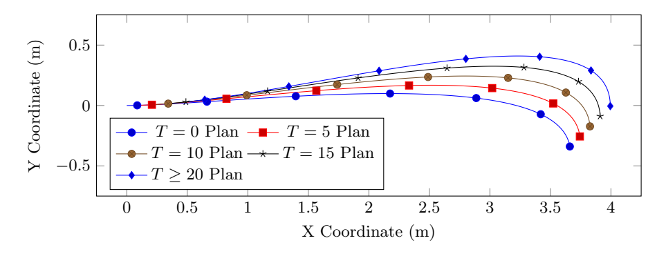
This QP can then be solved using a convex optimization algorithm, such as the active-set method implemented in qpOASES [4]. In this planning method, the planner is told to find a solution with horizon T. If it is possible to reach the goal state within time T, the solution to the above problem will be exactly the solution to the unconstrained problem. Otherwise, it will be a "best-estimate" solution. If the solution is exact, it can be followed to completion. If it is inexact, only the first step of the plan (some amount of time dt) will be followed, after which it will be replanned with the same horizon, effectively planning a path from time dt to time T+dt.

Fig 17 shows several iterations of the algorithm run from different timesteps. At T < 20, the problem is infeasible with the given horizon and so best-effort minimal solutions are found. When T ≥ 20, the problem is feasible and the robot does not need to replan, only follow the previous solution.

3.3 Torque Based Motion Control

Background

Torque control allows for better dynamic behavior, full motor torque capability at low speeds, and higher efficiency because of the decoupled control of rotor flux and torque. Torque control can be implemented on a BLDC motor through controlling a current directly responsible for the torque. Current in a BLDC motor is normally viewed in a stationary reference frame. To control the torque directly, the dq transform, described below, is applied. The motors used (Maxon 45 flat 42.8mm, brushless, 50 Watt, with Hall Sensors) have 3 windings that are configured in the wye configuration. A BLDC motor has three different voltage inputs that need to be supplied to control the motor. Our setup only requires a single voltage that is passed into an FPGA which converts the voltage into the 3-phase input. BLDC motors generate back EMF, but unlike AC synchronous motors which generate a sinusoidal back EMF, a BLDC motor has a trapezoidal back EMF.

Physical and Mathematical Foundations

Each winding needs to be supplied its own current for optimal operation. The currents are ia, ib, and ic. Fig. 18 shows the three different winding currents in a BLDC motor.

Eqs. 16 and 17 can be derived from Kirchhoff's Voltage Law: summing the voltage loss due to the resistance and inductance and subtracting the back EMF. Then, rather than using the third equation for voltage (from the third winding), we will use the fact that all the currents need to sum to 0, otherwise the three equations would all be linearly dependent. This results in Eq. 18.

$$v_{ab} = R(i_a - i_b) + L\frac{d}{dt}(i_a - i_b) + (e_a - e_b)$$ (16)

$$v_{bc} = R(i_a + 2i_b) + L\frac{d}{dt}(i_a + 2i_b) + (e_b - e_c)$$ (17)

$$i_a + i_b + i_c = 0$$ (18)

R is the resistance in the motor, L is the inductance, and ea, eb, and ec are the back EMF in the windings. The back EMF of each winding is a trapezoid defined by the Eqs. 19 - 21. ke is the back EMF constant of the motor. F() is a piecewise function that defines the trapezoid. This is given in Eq. 22. θe is the angle of the rotor.

$$e_a = \frac{k_e}{2} \omega F(\theta_e)$$ (19)

$$e_b = \frac{k_e}{2} \omega F(\theta_e - \frac{2\pi}{3})$$ (20)

$$e_c = \frac{k_e}{2} \omega F(\theta_e - \frac{4\pi}{3})$$ (21)

$$F(\theta_e) = \begin{cases} 1 & 0 \le \theta_e < \frac{2\pi}{3} \ 1 - \frac{6}{\pi} (\theta_e - \frac{2\pi}{3}) & \frac{2\pi}{3} \le \theta_e < \pi \ -1 & \pi \le \theta_e < \frac{5\pi}{3} \ -1 + \frac{6}{\pi} (\theta_e - \frac{5\pi}{3}) & \frac{5\pi}{3} \le \theta_e < 2\pi \end{cases}$$ (22)

The mechanical equation that defines this system is shown in Eq. 23 where Te is the electrical torque, Tl is the load torque, J is the inertia of the rotor, ω is the rotational velocity, and kf is the coefficient of viscous friction.

$$T_e = k_f \omega_m + J \frac{d\omega_m}{dt} + T_l = \frac{k_t}{2} [F(\theta_e)i_a + F(\theta_e - \frac{2\pi}{3})i_b + F(\theta_e - \frac{4\pi}{3})i_c]$$ (23)

Solving Eqs. 16, 17, and 23 for the derivatives of the state variables yields Eq. 24 and 25 which is a usable state space formulation for the motor dynamics.

$$\begin{bmatrix} i_a' \ i_b' \ \omega' \end{bmatrix} = \begin{bmatrix} -\frac{R}{L} & 0 & 0 \ 0 & -\frac{R}{L} & 0 \ 0 & 0 & -\frac{k_f}{I} \end{bmatrix} \begin{bmatrix} i_a \ i_b \ \omega \end{bmatrix} + \begin{bmatrix} \frac{2}{3L} & \frac{1}{3L} & 0 \ -\frac{1}{3L} & \frac{1}{3L} & 0 \ 0 & 0 & \frac{1}{I} \end{bmatrix} \begin{bmatrix} v_{ab} - e_{ab} \ v_{bc} - e_{bc} \ T_e - T_L \end{bmatrix}$$ (24)

$$\begin{bmatrix} i_a \ i_b \ i_c \ \omega \end{bmatrix} = \begin{bmatrix} 1 & 0 & 0 \ 0 & 1 & 0 \ -1 & -1 & 0 \ 0 & 0 & 1 \end{bmatrix} \begin{bmatrix} i_a \ i_b \ \omega \end{bmatrix}$$ (25)

Eq. 26 gives the equation of the dq transform where the abc frame is being transformed into the rotating dq frame. $\theta$ is the angle of the rotor and N is the number of poles.

$$\begin{bmatrix} i_d \ i_q \ i_0 \end{bmatrix} = \sqrt{\frac{2}{3}} \begin{bmatrix} \cos(N\theta) & \cos(N\theta - \frac{2}{3}\pi) & \cos(N\theta + \frac{2}{3}\pi) \ -\sin(N\theta) - \sin(N\theta - \frac{2}{3}\pi) - \sin(N\theta + \frac{2}{3}\pi) \ \frac{1}{\sqrt{2}} & \frac{1}{\sqrt{2}} \end{bmatrix} \begin{bmatrix} i_a \ i_b \ i_c \end{bmatrix}$$ (26)

Control

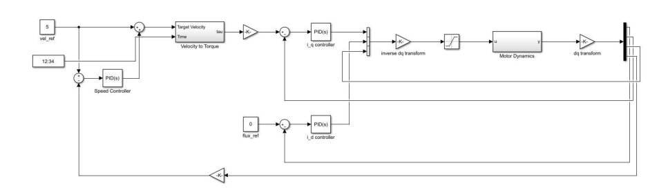
To control the brushless DC motor, Field Oriented Control (FOC) will be implemented [6]. In this technique, currents going to each of the windings in the stator will be individually controlled such that the optimal torque is produced. After applying the dq transform to the system, the system's inputs can be viewed as two independent currents, which can each be individually controlled. Due to the transformation, each current corresponds to a physical aspect of the motor: the $i_d$ current will control the flux in the motor, and the $i_q$ current has direct control over the torque produced by the motor. A rigorous mathematical proof of this can be found in [7]. The $i_d$ and $i_q$ currents must be transformed into the abc reference frame so they can be applied to the motor. This whole system is shown in Fig. 19.

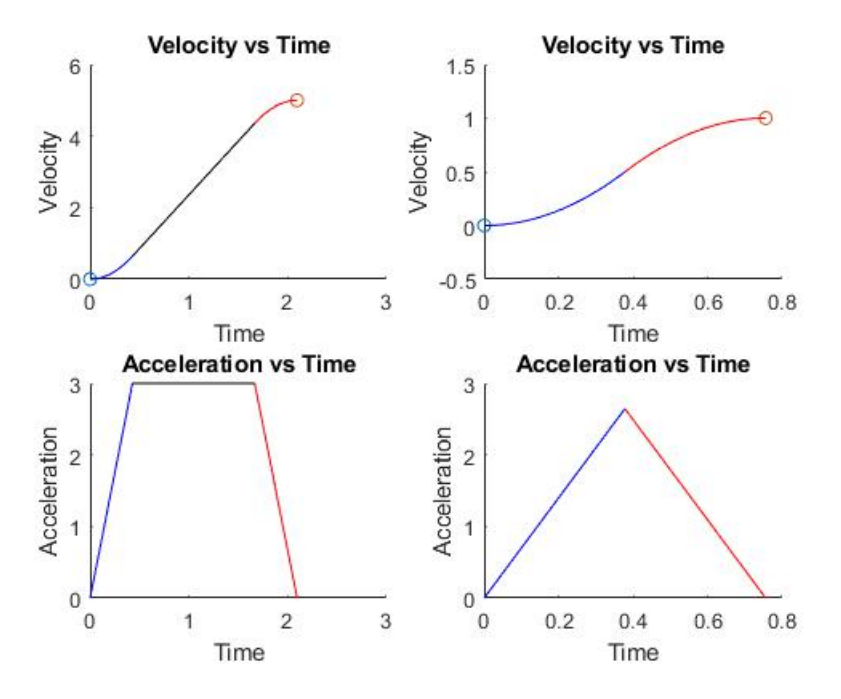
The state space formulation developed in Section 1 will be used for the motor dynamics. The simulation in Simulink is shown in Fig. 19. As you can see from Fig 19. there are 3 different control loops: speed control, torque control, and flux control. This control system architecture uses torque control, but the paths generate a velocity profile, so a trapezoidal acceleration profile is created given the target velocity. The target velocity that is passed into the torque generation function is created using PID on a feedback loop and a feedforward command. After the target torque is created, the torque is converted to the iq current. A PID loop acts on this current; this is the torque control. To create the id current, a reference value of 0 is used, this is explained in more depth below. A PID loop on the error between the measured id and the desired value is used to minimize error. The vd and vq voltages are transformed into the abc frame and used as inputs to the motor. The measured current are transformed from the abc frame to the dq and used for feedback along with the speed.

By setting idref to 0, the back EMF is minimized which maximizes the torque for the given power supplied. If the idref current is set higher, then the field strength will increase which will increase the back EMF. This would decrease the torque and increase the speed and is called the "field weakening zone". If the goal was to run at higher speeds with the same power draw then control of idref would be necessary, but for this application that is unnecessary [8].

Velocity to Torque Profile Generation

Given a starting velocity, v0 and a target final velocity vf, a followable trapezoidal acceleration profile will be created. Using motor constraints such as maximum acceleration and jerk, a time efficient equation for the motion can be derived. It is possible that the commanded change in velocity is too small to reach steady state acceleration and thus a triangular acceleration profile will be more optimal. In this case the robot will move at maximum jerk for the first half of the profile, then move to negative maximum jerk for the second half. In the trapezoidal case the acceleration will change at maximum jerk to create the first part of the trapezoid. Then, upon reaching maximum acceleration, the robot will move at this acceleration until it needs to decelerate. Then the robot will move at negative maximum jerk until it reaches zero acceleration and it is at vf. This results in an s-curve velocity profile, and an acceleration profile that starts and ends at zero acceleration. Fig. 20 shows an example of generated profile.

4 Open Source

4.1 Open-Source Software

RoboJackets open sources the entire software stack. The camera filters, AI, higher level motion control, and path planning can be found online. The code contains low level documentation through the use of Doxygen with high level overviews and training slides found in the RoboJackets training section. The level of documentation allows others to easily use and understand the code base without fully dissecting the entire RoboCup implementation.

4.2 Open-Source Platform

For the first time, RoboJackets has open sourced its mechanical platform in addition to PCBs, firmware, and build systems. This addition means its platform is now completely open source. In addition, subsystem design analysis documents were created. After talking with other teams, kicker boards appear to be a reliability and performance pain point. To help alleviate this, a detailed analysis document was created, within which every RoboJackets kicker board design since 2013 is analyzed for failure points based on alumni testimony and commit logs. This helped refine the work for the new version, and should serve as an excellent summary of pitfalls for new teams.

4.3 Usage

All files and documentation can be found at its FOSS portal [9]. Everything is licensed liberally under Apache 2.0 or Creative Commons 3.0. Feel free to use these resources as you see fit. We welcome all contributions.

5 Acknowledgements

M. Akhtar, T. Jones, A. Khadse, R. Medrano, A. Penkar, D. Yang

References

1. ZJUNlict. ZJUNlict RoboCup SSL Fleet 2018. National Laboratory of Industrial Control Technology.
2. Oliver Birbach Mahisorn Wongphati Manuela Veloso Stefan Zickler, Tim Laue. Sslvision: The shared vision system for the robocup small size league.
3. Qian Qian. Multi-Hypotheses Kalman Filter based Self-Localization for Autonomous Soccer Robots. Master's thesis, Technische Universität Berlin, July 2015.
4. C. Kirches H.J. Ferreau, A. Potschka. qpOASES webpage. http://www.qpOASES.org/, 2007–2017.
5. M. A. Awadallah, Ehab H. E. Bayoumi, Hisham Soliman. Adaptive deadbeat controllers for brushless DC drives using PSO and ANFIS techniques. Journal of Electrical Engineering, 60(1):3–11, 2009.
6. Pter Dr. Korondi, Krisztin Dr. Samu, Levente Raj, Annamria Dcsei-Parczi, Dnes Dr. Fodor, Jzsef Dr. Vsrhelyi, Jzsef Dr. Vass. Digital Servo Drives, chapter 5. BME MOGI, 2014.
7. David G. Taylor. Modeling and Analysis of AC Motor Drive Systems. ECE 4550 Class Notes, 2014.
8. B.P. Singh Mukesh Kumar, Bhim Singh. Modeling and Simulation of Permanent Magnet Brushless Motor Drives using Simulink, 2002.
9. RoboJackets RoboCup SSL Team. RoboJackets SSL FOSS Portal, 2019. https://robojackets.github.io/robocup.