TIGERs Mannheim (Team Interacting and Game Evolving Robots) - Extended Team Description for RoboCup 2019
Nicolai Ommer, Andre Ryll, Mark Geiger
Department of Information Technology Baden-Württemberg Cooperative State University, Coblitzallee 1-9, 68163 Mannheim, Germany
Abstract This paper presents a brief overview of the main systems of TIGERs Mannheim, a Small Size League (SSL) team intending to participate in RoboCup 2019 in Sydney, Australia. This year, the ETDP will provide details on our path planning algorithm, which is rather distinct in the league and is used by our team for several years now. Furthermore, the rating functions for good pass locations are outlined. They are a major part of our pass-oriented play style. Additionally, we will briefly introduce our new robot design, which is developed from scratch.
1 Mechanical and Electrical System
This year we are developing our fourth iteration of our robot hardware. This generation is redesigned from scratch and features higher motor power, more sensors, and the option for an onboard compute model. A comparison of our current v2016 model and the next generation v2019 is shown in table 1.
The drive train has been updated from 50W motors to 70W motors. Furthermore, the encoders have been changed from optical ones to magnetic ones which provide a higher resolution and dirt resistance. The wheel size has been reduced by 32% to be able to arrange all wheels with 90° spacing. This significantly reduces friction effects and eases motion control. The dribbling motor has been exchanged for a lighter Maxon ECX Speed 13L. The new motor runs a much higher speeds, hence a two-step gear is required to achieve optimal performance at 15000rpm.
The primary microcontroller has been updated to a STM32H743 running at 400MHz. Furthermore, five STSPIN32F0A microcontrollers replace the Allegro A3930 ICs for individual motor control. An additional STM32F031 handles processing the front infrared barrier for ball detection. All secondary microcontrollers are connected to the primary one via individual serial connections (UART). In addition to the v2016 sensors, the new version now also employs a compass for absolute heading measurements.
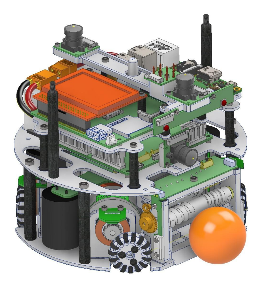
Table 1: Robot Specifications
| Robot version | v2016 | v2019 |
|---|---|---|
| Dimension | Ø179 x 146mm | Ø178 x 146mm |
| Total weight | 2.5kg | 2.5kg |
| Max. ball coverage | 19.7% | 19.3% |
| Driving motors | Maxon EC-45 flat 50W | Maxon EC-45 flat 70W¹ |
| Gear | 18 : 60 | 30 : 50 |
| Gear type | Internal Spur | External Spur |
| Wheel diameter | 57mm | 33mm |
| Encoder | US Digital E8P, 2048 PPR [1] RLS RLC2HD, 36864ppr [2] | |
| Dribbling motor | Maxon EC-max 22 | Maxon EXC Speed 13L HP |
| Dribbling gear | 50 : 30 | 12 : 32 + 14 : 18 |
| ØDribbling bar | 14mm | 12mm |
| Kicker topology | Flyback Converter (up to 230V) | |
| Chip kick distance | approx. 2.5m | approx. 3m |
| Straight kick speed | max. 8m/s | max. 8.5m/s |
| Microcontroller | STM32F746 [3] | STM32H743 [4] |
| Sensors | Encoders, Gyroscope, Accelerometer |
Encoders, Gyroscope, |
| Accelerometer, Compass, | ||
| Cameras, Microphones | ||
| Communication link | Semtech SX1280 @1.3MBit/s, 2.300 - 2.555GHz [5] | |
| Compute module | N/A | Raspberry Pi 3 or nVidia |
| Jetson TX2 | ||
| Onboard cameras | N/A | 1 front, 2 up |
The v2019 robots have been specifically designed for more autonomy by having space for a compute module. They can either be equipped with a Raspberry Pi 3 with one front looking camera or with a Jetson TX2 with up to three cameras (one front, two up). The front camera will be used for ball detection. The two upward facing stereo cameras can be used for visual odometry to provide an alternative position source for the official SSL-Vision.
Figure 1 shows a CAD rendering of the new robot. v2016 and v2019 robots use the same wireless link and protocol, hence they are transparent to our central AI software allowing us to run heterogeneous teams in case we need to use old and new robots.
Further tests need to be done in order to evaluate the usefulness of enhanced (encoders) and new (compass, cameras, microphones) sensors. At the time of writing they have only been integrated in hardware but are not used yet in software.
¹ Alternative option: Nanotec DF45L024048-A2, 65W
2 Path Planning
This year, the software section focuses on the robot control, including path planning, trajectory generation and execution on the robot. A common path planning approach is the Rapidly-exploring random tree (RRT) algorithm which is widely employed in the SSL. However, some years ago we replaced our RRT algorithm with a custom algorithm. It searches for paths by generating trajectories. Collisions are detected by stepping over them. The trajectories are the same we use on our robots for motion control. The advantage is that the resulting trajectory path can be executed by the robots, while with RRT, another post processing is required to get a physically reasonable trajectory from a path. Additionally, we gain information on the time until a robot reaches its destination and we can better coordinate our own robots because we know the robot positions over time quite precisely.
The following sections will start with some preliminary information about the system we use and the constraints we have, before explaining the path planning algorithm in detail.
2.1 Trajectories
Our robot control is based on two-dimensional bang bang trajectories for the translative movement with velocity limits and fixed acceleration. The orientation is controlled separately. The two dimensions are synchronized such that both one-dimensional trajectories use approximately the same time [6]. One of the limitations of the trajectory generation is that the end velocity must be zero. This was a major constraint in the design of the path planning algorithm which had to be considered. Though, any other trajectory should theoretically also work, as long as it can be generated from an initial position and velocity and a final position.
2.2 Robot control
The robot control of our team is rather distinct in the league, yet. Most teams send velocities to their robots and thus have at least one control loop in their central software. In contrast to that we send a destination to our robots. A dedicated base station receives and forwards the SSL-Vision position to each robot. The communication with our robots is described in details in the ETDP from 2016 [7]. The robot can drive to the given destination without any further updates from our software.
The path planning, however, is done in our software. In order to avoid obstacles we need to find an alternative intermediate destination that maneuvers the robot around the upcoming obstacles. The destination could be updated in each frame, but in order to achieve a smooth, precise, and independent movement, the intermediate destination should be as stable as possible. This is considered during path planning by preferring the last intermediate destination.
The robot control in the software is performed in so called skills, most of which make use of path planning. Skills are updated with 100Hz with one thread per robot. They take the current positions and velocities of all objects from our internal vision filter and update the match (control) command of their designated robot at the end. The updated match command is sent to the base station [7].
2.3 Path planning algorithm
Given a destination, a set of obstacles and some movement limits and constraints, the path planning algorithm will find exactly one trajectory. The trajectory is not necessarily optimal and it may have collisions. In a quickly changing environment like the SSL we have to find a trade-off between optimal paths and calculation time. We prefer to find a valid path within one time step (10ms) so that we can react to fast moving opponent robots as quickly as possible. A collision one second or more in the future is fine, if no other path can be found in the current time step. The obstacle might be gone in the next time step anyway.
The algorithm will first generate a trajectory to the destination and check if there is a collision on this trajectory. If not, it will stop here and return this trajectory. Otherwise, it will generate a fixed number of trajectories. The way of generating these trajectories is described in the upcoming sections. A collision check is performed on each of these trajectories by stepping over them in 100ms steps. Stepping stops after a fixed amount of time (3s).
Afterwards, each trajectory gets a penalty score. Given $t_{total}$ is the total trajectory time, $t_{cl} = 3.0s$ is the collision lookahead until which a collision is considered, $t_{cdf}$ is the collision duration on the front of the trajectory and $t_{fc}$ is the time when the first collision occurs, multiple penalties are considered:
– Total trajectory time: prefer faster trajectories
$$P_{totalTime} = t_{total} \tag{1}$$
– Collision on trajectory (fixed 5s penalty): avoid collisions
$$P_{collision} = \begin{cases} 5.0 & collision_present \ 0.0 & otherwise \end{cases} \tag{2}$$
– Distance [m] between position at collision check limit (3s) and destination: improve paths, if destination is far away
$$P_{farCollision} = \begin{cases} max(0, |p_l - p_d|) & t_{total} >= t_{cl} \ 0.0 & otherwise \end{cases} \tag{3}$$
– Time until first collision: Prefer trajectories with collisions farther away
$$P_{firstCollision} = \begin{cases} max(0, t_{cl} - t_{fc}) & intermediate_collision_present \ 0.0 & otherwise \end{cases} \tag{4}$$
– Collision duration on front of trajectory: trajectories with less front duration leave the obstacle faster
$$P_{frontCollision} = \begin{cases} 0.0 & always_colliding \ 3t_{cdf} & otherwise \end{cases} \tag{5}$$
The total penalty score is the sum of all scores:
$$P_{total} = P_{totalTime} + P_{collision} + P_{farCollision} + P_{firstCollision} + P_{frontCollision} \tag{6}$$
The trajectory with the lowest penalty score is considered the best one of the current iteration. One extra trajectory is generated with the intermediate destination of the last iteration. If the penalty score of this trajectory is significantly larger then the one of the best new one, the new trajectory is returned. Otherwise, the trajectory of the intermediate destination from the last iteration is returned.
2.4 Generating trajectories based on intermediate destinations
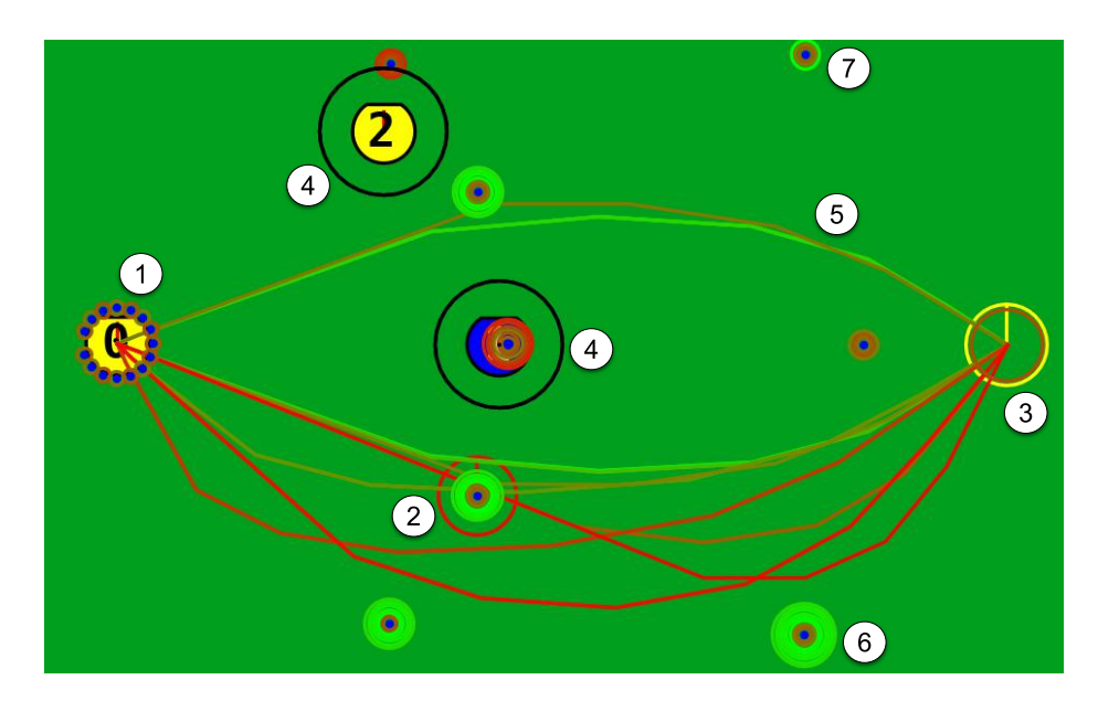
Trajectories are generated from a fixed number of intermediate destinations around the current robot position. They can either be generated randomly, or in a systematic way. The latter has the advantage of more predictable results, while the randomness might help avoiding to get stuck. Experiments have not shown significant differences, though. We used the systematic generation during RoboCup 2018.
2.5 Modeling obstacles
Obstacles are not static shapes, but can depend on time. The path planning algorithm takes a list of obstacles as input. Each obstacle implements one method:
$colliding(point : Vector2, time : double) : boolean$
Simple obstacles, like defense area, field borders and the restricted area around a ball are not time dependent and are only modeled as rectangular or circular shapes. Our own robots are modeled using their current trajectory. The margin depends on the velocity on the trajectory. If a robot is moving fast the margin is larger then when a robot is moving slowly. The opponent robots are modeled as a circle shifted towards the moving direction. The circle reflects the theoretical action space of the opponent based on a fixed acceleration motion model. The ball is modeled using a ball trajectory. The ball trajectory is based on the two-phase ball model, presented by ER-Force in their 2016 ETDP [8].
2.6 Optimizations
Several optimizations, introduced over the years, have been applied to the basic algorithm. They are outlined in this section.
Collision checks are only performed until a fixed maximum time (3 seconds). There are two major reasons for this. Firstly, most obstacles are moving robots and balls. The longer we look into the future, the less likely it is that we have predicted the state of these obstacles correctly. There is also plenty of time to react on those obstacles later. Ignoring these obstacles simplifies the path because it can focus on the critical time horizon while being only modeled by a single intermediate destination. Secondly, this also limits the maximum processing time. Large peaks in the processing time should be avoided for a smooth and fast reacting movement.
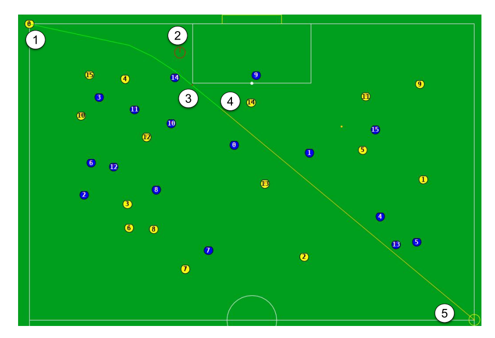
The current robot position or the destination could be inside an obstacle. In this case, there would be no collision free trajectory and the path planning would not work well. To solve this the duration of the front and back collision on the trajectory is also considered in the penalty score and the first collision time is calculated starting from the first non collision time step on the trajectory.
The accuracy of the trajectory heavily relies on the robot state (position and velocity). However, due to the system delay we do not know the current state of our robots. Instead of predicting this state based on measured data we simply assume that the robot moves exactly on the trajectory that we calculated in the previous step. It is only reset if the measured position significantly differs from the trajectory position. That way there are no issues with delays in the state and imprecise measurements.
As mentioned in section 2.3 the path planning algorithm may return a trajectory with a collision on it. Depending on the time to the collision and the type of obstacle the velocity limit is reduced significantly first. If it gets too close and our robot is fast an emergency brake is applied. This is a special command that is also used during HALT and will bring the robot to a stop as fast as possible.
When coordinating multiple robots it can happen that both robots try to avoid each other in a symmetric way and push each other away from their destinations. To avoid this a priority map is applied. Each robot has a different priority. Robots with a higher priority neglect the robots with a lower priority. In a match the priorities are populated from the roles that the robots have. Otherwise, the robot IDs are taken as a default.
2.7 Evaluation
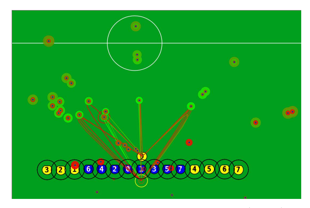
The idea of an alternative path finder, that is not based on RRT, was introduced in 2015. Since then, it has been evolved to what is described in this paper. At RoboCup 2018 automatic referees had checked for collisions throughout all games for the first time. We were one of the teams with the fewest collisions throughout the tournament. This shows that our approach works well in avoiding collisions.
One of the main constraints of the path planning algorithm is the processing time. In the previous sections it was already mentioned that there are some limits to avoid unpredictably long processing time. The processing time primary depends on the number of intermediate destinations that are generated. That is why those are fixed. Additionally, it depends on the number of obstacles. At each time step on a trajectory a collision check is performed for each obstacle. Luckily, the number of obstacles is also limited to the number of objects on the field. The trajectories are a crucial part in the processing time. For one robot about 35.000 trajectories are generated per second. Hence, the cost for this generation has to be cheap.
2.8 Next steps
One of the next steps is to find another trajectory type that is even better suited for our robot control but could still be used with the path planning algorithm. While we are basically satisfied with bang bang trajectories we are still looking for trajectories that better adapt to the physical limits of our robots.
3 Pass target rating
In the past years we worked on improving our pass-focused play style. In our 2017 ETDP [9] we explained the concept of pass targets and pass synchronization. This concept was also used during RoboCup 2018 with some minor improvements. In this section the calculation of the pass target score(s) is explained. Note that the generation of pass target locations is not part of this section an can be looked up in [9].
3.1 Previous approaches
Until RoboCup 2018 each pass target T had exactly one score associated with it. This score was based on numerous probabilities like goal chance, pass interception hazard, overall pass distance, etc. Let us denote the individual probabilities as $p^i$ where i ranges from 0 to n, the total number of probabilities taken into account. Then the final score $s_{total}$ is calculated as:
$$s_{total} = \sum_{i=0}^{n} w_i \cdot p_i \tag{7}$$
Where $w^i$ denotes individual weights per considered probability. The probability values are bounded between the values zero and one, with the general meaning of being bad towards zero and good towards one. Here, the problem with our previous approach becomes visible. First of all, it is very susceptible to tuning errors. Let us assume there is a probability for a successful pass $p_{pass}$ and an associated weight $w_{pass}$. Due to the fact that $p_{pass}$ approaches a probability of one it may dominate over all other probabilities. This leads to endless sequences of pass play. This could be countered by adjusting $w_{pass}$ but selecting a wrong magnitude for the weight may also lead to no passes being made at all.
Furthermore, only one pass target score is used for all situations whereas it may be desirable to adjust them depending on situation. With the given approach this leads to multiple sets of $w^i$ making tuning even more error-prone.
3.2 "One score, one strategy" rating
Instead of using one single score $s_{total}$ for all pass targets we decided to split up the score into multiple strategy-oriented scores. During RoboCup 2018 we used two distinct scores. One score denoted the probability to shoot a goal from the pass target location. We call this a redirect goal as the ball is passed to a robot and then redirected into the goal. Hence, let us denote this score as $s_{rgoal}$. The second score simply denotes the probability to receive a pass and stop the ball. We denote this score as $s_{pass}$. $s_{rgoal}$ and $s_{pass}$ are always computed for all pass targets T. If we denote $G = {T | s_{rgoal} > 0}$ then the best pass target $T_{best}$ is computed by:
$$T_{best} = \begin{cases} max_T (s_{pass}) & G = \emptyset \ max_T (s_{rgoal}) & otherwise \end{cases} \tag{8}$$
This means that we will use $s_{rgoal}$ as soon as there is a pass target with a chance to shoot a goal. This aligns with the main objective of the game. If this is not possible, we favor game control and ball possession and select the best possible pass to a friendly robot.
Having two distinct scores also simplifies tuning and adds robustness. If passes are intercepted too often, this probability can be weighted higher without affecting goal shots. Thereby, we could select to play safe passes but very risky goal shots. Furthermore, misadjusting a weight can no longer negatively impact the complete pass target rating.
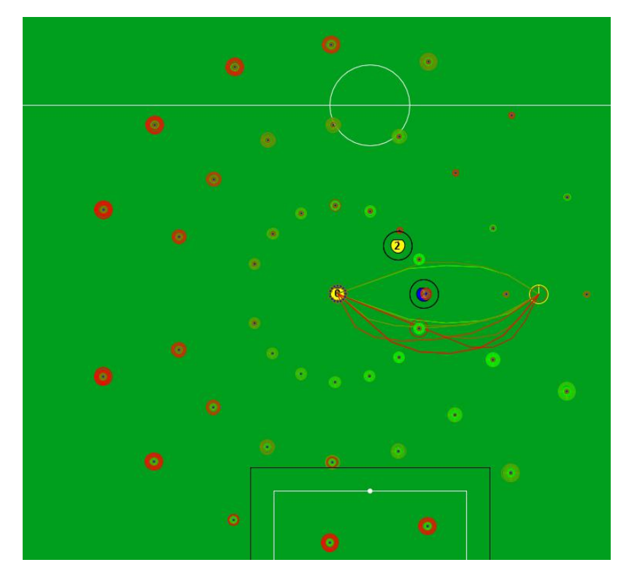
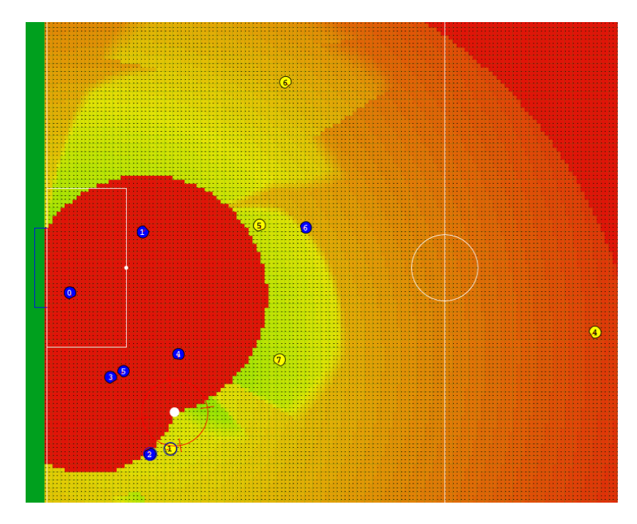
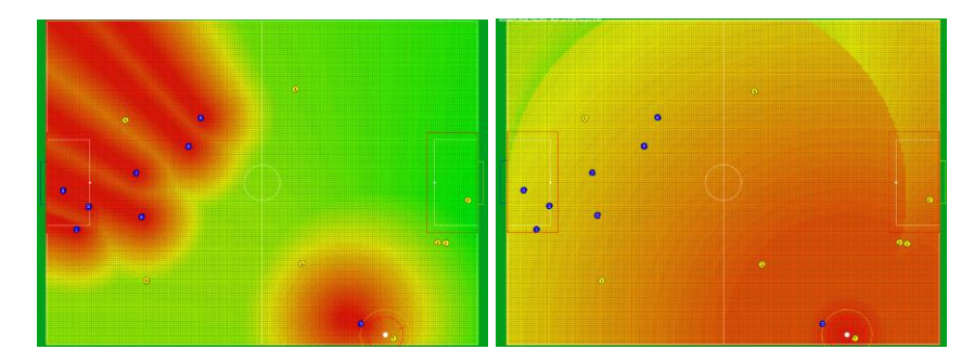
Redirect Goal Shot Score The redirect goal short score $s_{rgoal}$ is a combination of several criteria: The redirect angle, the overall distance of the pass and goal shot, the pass success probability and the goal shot success probability. Figure 6 shows how the score looks for every point on the field for one specific scenario. The most dominant and most important criteria is the redirect angle $\alpha$. The redirect angle is the angle between the ball position, the pass target and the opponents goal. If a redirect is not possible then the overall score is automatically zero (deep red dots in figure 6). The criteria are mapped to probabilities as follows:
$$p_{angle} = 1 - rel\left(\alpha, 45^{\circ}, \alpha_{max}\right) \tag{9}$$
$$p_{dist} = 1 - rel\left(d, 0, d_{max}\right) \tag{10}$$
with:
$$rel(x, min, max) = \begin{cases} 1 & x \ge max \ \frac{x - min}{max - min} & min < x < max \ 0 & x \le min \end{cases} \tag{11}$$
Where $\alpha_{max}$ defines the maximum acceptable redirect angle, $d$ the distance from pass origin to pass target and from there to the goal, and $d_{max}$ the maximum total distance acceptable for d. Angles smaller than 45° have a maximum $P_{angle}$ score. Furthermore, the pass success probability $p_{pass}$ is defined by the width of the free corridor from the pass origin to the pass target. Goal success probability $p_{goal}$ has been described in detail in our 2017 ETDP [9] (section 2.2 "The Score Chance").
3.3 Results
The "one score, one strategy" rating showed good results during RoboCup 2018. It is easier to control and easier to maintain than the previous approaches. Mostly because now the redirect goal shot and pass scores can be tweaked independently from each other, without effecting the behavior of the other strategy score.
One of the next steps is to add a new strategy, thus also a new strategy score for intermediate pass positions. This can be very important if the field size is increased again. The new strategy should represent some kind of mid-field play, that will be more important when the field size increases.
4 Publication
Our team publishes all their resources, including software, electronics/schematics and mechanical drawings, after each RoboCup. They can be found on our website. The website also contains several publications with reference to the RoboCup, though some are only available in German.
References
- US Digital. E8P OEM Miniature Optical Kit Encoder, 2012. http://www.usdigital.com/products/e8p
- RLS, A Renishaw associate company. RLC2HD Datasheet, September 2017. https://www.rls.si/en/fileuploader/download/download/?d=0&file=custom%2Fupload%2FRLCD03_03RLC2HD_datasheet.pdf
- STmicroelectronics. STM32F745xx, STM32F746xx Datasheet, December 2015. http://www.st.com/st-web-ui/static/active/en/resource/technical/document/datasheet/DM00166116.pdf
- STmicroelectronics. STM32H743xI Datasheet, July 2018. https://www.st.com/resource/en/datasheet/stm32h743bi.pdf
- Semtech Corporation. SX1280 Datasheet, May 2017. http://www.semtech.com/images/datasheet/sx1280_81.pdf
- O. Purwin and R. D'Andrea. Trajectory generation for four wheeled omnidirectional vehicles. In Proceedings of the 2005, American Control Conference, 2005., pages 4979–4984 vol. 7, June 2005.
- A. Ryll, M. Geiger, N. Ommer, A. Sachtler, and L. Magel. TIGERs Mannheim - Extended Team Description for RoboCup 2016, 2016.
- C. Lobmeiner, P. Blank, J. Buehlmeyer, D. Burk, M. Eischer, A. Hauck, M. Hoffmann, S. Kronberger, M. Lieret, and M. Eskofier. ER-Force - Extended Team Description for RoboCup 2016, 2016.
- M. Geiger, C. Carstensen, A. Ryll, N. Ommer, D. Engelhardt, and F. Bayer. TIGERs Mannheim - Extended Team Description for RoboCup 2017, 2017.